Archive for category research
Favorite Artists vs Distinctive Artists by State
In my recent regional listening preferences post I published a map that showed the distinctive artists by state. The map was rather popular, but unfortunately was a source of confusion for some who thought that the map was showing the favorite artist by state. A few folks have asked what the map of favorite artists per state would look like and how it would compare to the distinctive map. Here are the two maps for comparison.
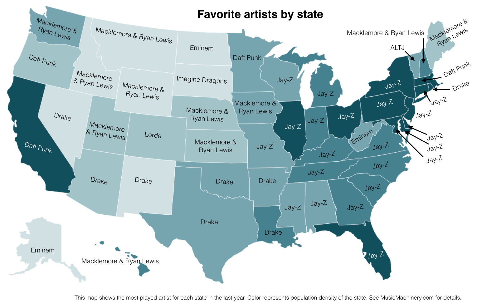
Favorite Artists by State
This map shows the most played artist in each state over the last year. It is interesting to see the regional differences in favorite artists and how just a handful of artists dominates the listening of wide areas of the country.
Most Distinctive Artists by State
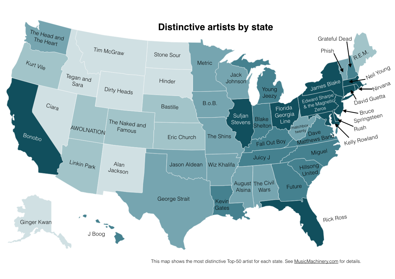
This is the previously published map that shows the artists that are listened to proportionally more frequently in a particular state than they are in all of the United States.
The data for both maps is drawn from an aggregation of data across a wide range of music services powered by The Echo Nest and is based on the listening behavior of a quarter million online music listeners.
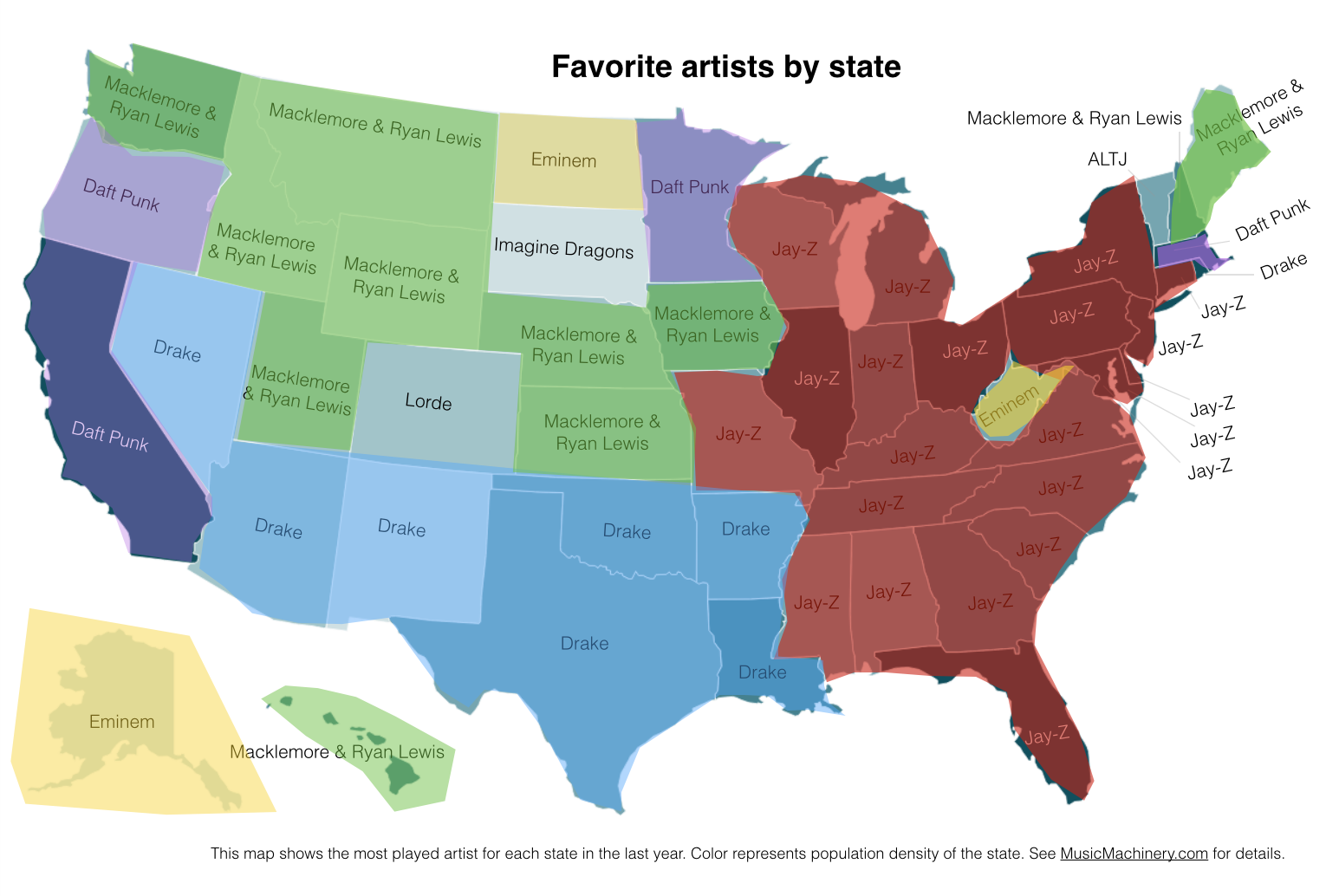
It is interesting to see that even when we consider just the most popular artists, we can see regionalisms in listening preferences. I’ve highlighted the regions with color on this version of the map:
Favorite Artist Regions
Exploring age-specific preferences in listening
Earlier this week we looked at how gender can affect music listening preferences. In this post, we continue the tour through demographic data and explore how the age of the listener tells us something about their music taste.
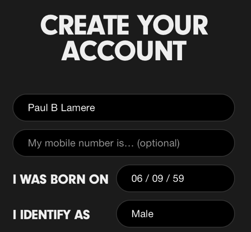
Where does the age data come from? As part of the enrollment process for most music services, the user is asked for a few pieces of demographic data, including gender and year-of-birth. As an example, here’s a typical user-enrollment screen from a popular music subscription service:
Is this age data any good? The first thing we need to do before we get too far with analyzing the age data is to get a feel for how accurate it is. If new users are entering random values for their date of birth then we won’t be able to use the listener’s age for anything useful. For this study, I looked at the age data submitted by several million listeners. This histogram shows the relative number of users by year of birth.
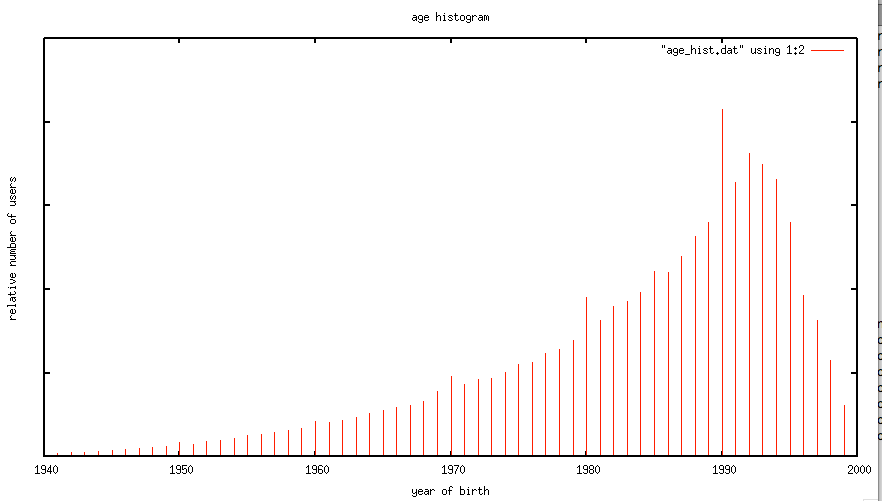
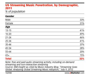
The first thing I notice is the curve has the shape one would expect. The number of listeners in each age bucket increases as the listener gets younger until around age 21 or so, at which points it drops off rapidly. The shape of the curve aligns with the data from this study by EMI in 2011 that shows the penetration of music streaming service by age demographic. This is a good indicator that our age data is an accurate representation of reality.
However, there are a few anomalies in the age data. There are unexpected peaks at each decade – likely due to people rounding their birth year to the nearest decade. A very small percentage (0.01 %) indicate that they are over 120 years old, which is quite unlikely. Despite this noise, the age data looks to be a valid and fairly accurate representation, in the aggregate, of the age of listeners. We should be able to use this data to understand how age impacts listening.
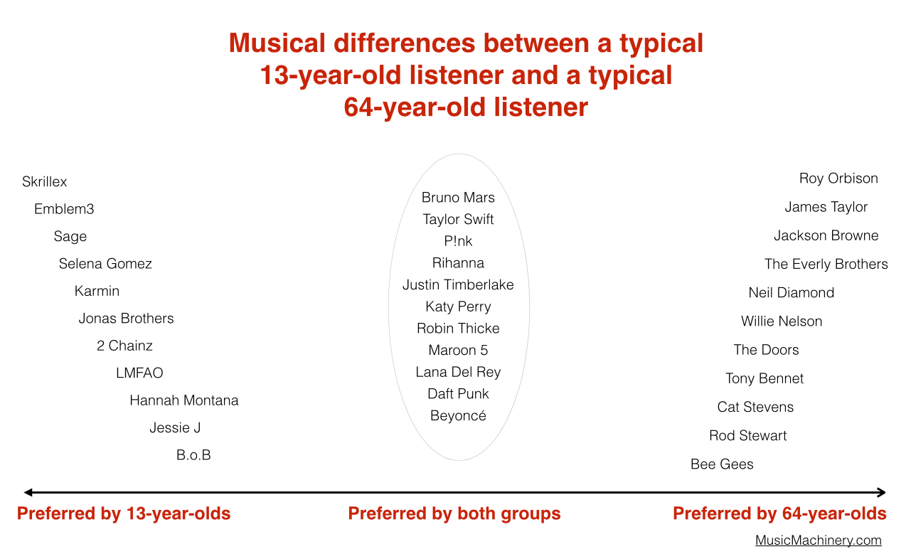
Does a 64-year-old listen to different music than a 13-year-old?
One would expect that people of different ages would have different music tastes. Let’s see if we can confirm this with our data. For starters, lets compare the average listening habits of 64-year-old listeners to that of the aggregate listening habits of the 13-year-old listener. For this experiment I selected 5,000 listeners in each age category, and aggregated their normalized artist plays to find the most-frequently-played artists. As expected, you can see that 64-year-old listeners have different tastes than 13-year-old listeners.
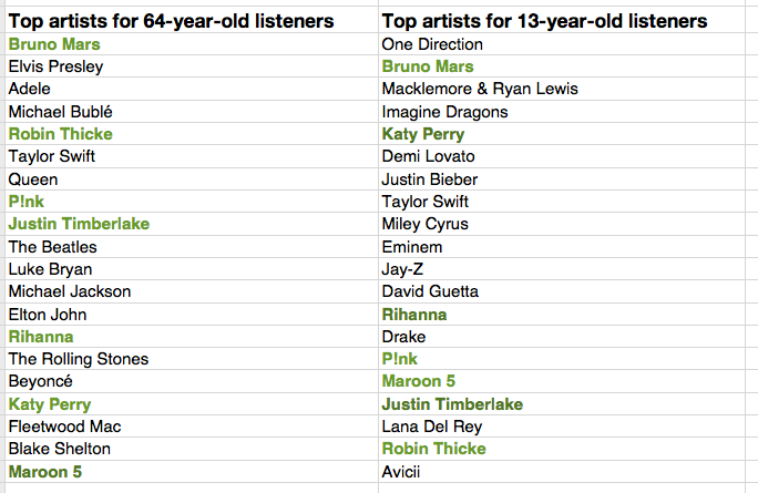
The top artists for the average 64-year-old listener include a mix of currently popular artists along with a number of artists from years gone by. While the top artists for the average 13-year-old includes only the most current artists. Still, there are seven artists (shown in bold) that overlap in the top 20 – an overlap rate of about 35%. This 35% overlap is consistent across all ranges of top artists for the two groups. No matter if we look at the top 100 or the top 1000 artists – there’s about a 35% overlap between the listening of 13- and 64-year-olds.

I suspect that 35% overlap is actually an overstatement of the real overlap between 13- and 64-year-olds. There are a few potential confounding effects:
- There’s a built-in popularity bias in music services. If you go to any popular music service you will see that they all feature a number of playlists filled with popular music. Playlists like The Billboard Top 100, The Viral 50, The Top Tracks, Popular New Releases etc. populate the home page or starting screen for most music services. This popularity bias inflates the apparent interest in popular music so, for instance, it may look like a 64-year-old is more interested in popular music than they really are because they are curious about what’s on all of those featured playlists.
- The age data isn’t perfect – for instance, there are certainly a number of people that we think are 64-years-old but are not. This will skew the results to artists that are more generally popular. We don’t really know how big this affect is, but it is certainly non-zero.
- People share listening accounts – this is perhaps the biggest confounding factor – that 64-year-old listener may be listening to music with their kids, their grand-kids, their neighbors and friends which means that not all of those plays should count as plays by a 64-year-old. Again, we don’t know how big this effect is, but it is certainly non-zero.
Let’s pause and have a listen to some music. First the favorite music of a typical 64-year-old listener:
And now the favorite music of a typical 13-year-old listener:
Finding the most distinctive artists
Perhaps more interesting than looking at how the two ages overlap in listening, is to look at how they differ – what are the artists that a 64-year-old will listen to that are rarely, if ever, listened to by a 13-year-old and vice versa. These are the most distinctive artists.
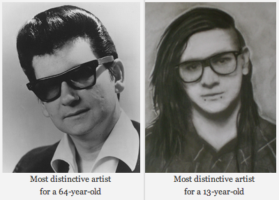
We can find the distinctive artists by identifying the artists in the top 100 of one group that fall the furthest in ranking in the other group. For example Skrillex is the 40th most listened to artist for the typical 13-year-old listener, but for 64-year-old listeners, Skrillex falls all the way to the 3,937 most listened to artist, making Skrillex one of the most distinguishing artist between the two groups of listeners. Likewise, Roy Orbison is the 42nd most listened to artist among 64-year-olds. He drops to position 4,673 among 13-year-olds making him one of the distinguishing artists that separate the 64-year-old from the 13-year-old.
We can use this technique to create playlists of artists that separate the 13-year-old from the 64-year-olds. Are you a 13-year-old, having a party and really wish that grandma would go to another room? Try this playlist:
Are you a 64-year-old and you want all of those 13 year-olds at the party to go home? Try this playlist:
We can also use this data to bring these two groups together. We can find the music that is liked the most among the two groups. We can do this by ordering artists by their worst ranking among the two groups. Artists like Skrillex and Roy Orbison fall to the bottom of the list since each is poorly ranked by one of the groups, while artists like Katy Perry and Bruno Mars rise to the top because they are favored by both groups.
Again, the confounding factors mentioned previously will bias the shared lists to more popular music. Nevertheless, if you are trying to make a playlist of music that will please both a 64-year-old and a 13-year-old, and you know nothing else about their music taste, this is probably your best bet.
Artists that are favored by both 64-year-old and 13-year-old listeners are: Bruno Mars, Taylor Swift, P!nk, Rihanna, Justin Timberlake, Katy Perry, Robin Thicke, Maroon 5, Lana Del Rey, Daft Punk, Beyoncé, Drake, Luke Bryan, Adele, Macklemore & Ryan Lewis, Miley Cyrus, David Guetta, Lorde, Jay-Z, Usher
We can sum up the differences between the two groups in this graphic:
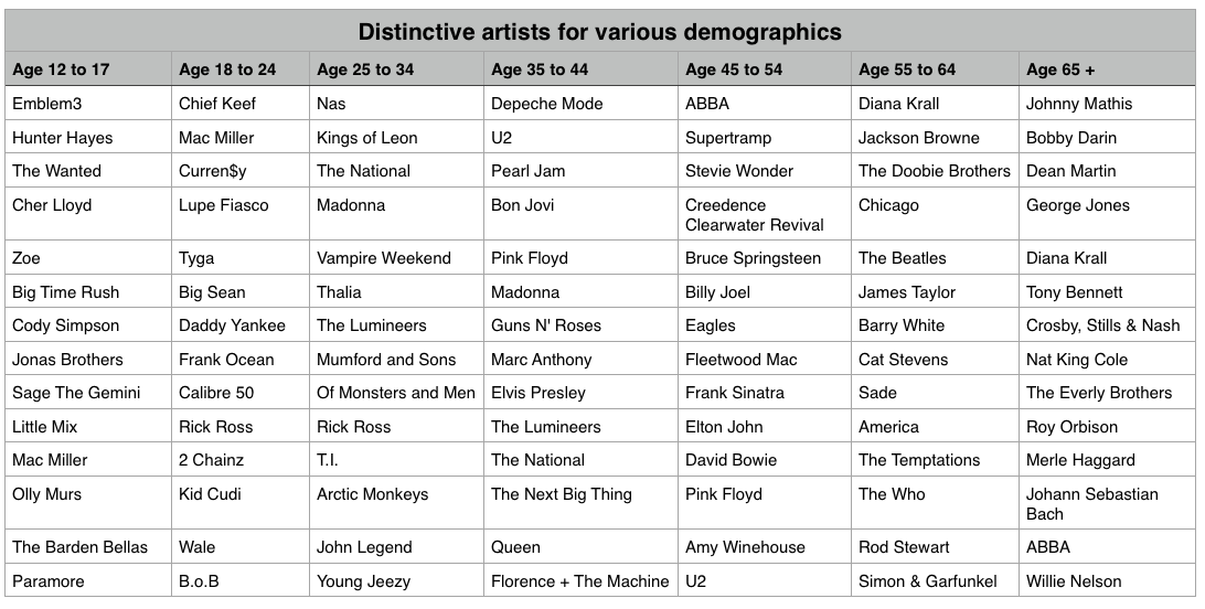
Broadening our view
We’ve shown that, as expected, 13-year-olds and 64-year-olds have different listening preferences. We can apply the same techniques across the range of age demographics typically used by marketers. We can find the most distinctive artists for each demographic bucket. It is interesting to see the progression of music taste over time. For instance, it is clear that something happens to a music listener between the 25 to 34 and 35 to 44 age buckets. The typical listener goes from hipster (Lumineers, Vampire Weekend, The National), to old (Pearl Jam, U2, Bon Jovi).
It is interesting to look at the starting year for artists in each of these buckets to get a sense of how the artist’s own age relates to the age of their fans:
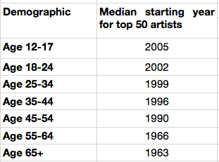
My take-way from this is that no matter how old you are, you don’t like the music from the 70s and the 80s so much.
Most homogenous Artists
We can also find the artists that are most acceptable across all demographics. These are the artists that are liked by more listeners in all of the groups. Like in the 13/64-year-old example, we can find these artists by ordering them by their worst ranking among all the demographic groups.
Most homogeneous artists: Bruno Mars, Rihanna, Katy Perry, Lana Del Rey, Beyoncé, P!nk, Jay-Z, Macklemore & Ryan Lewis, Daft Punk, Maroon 5, Justin Timberlake, Robin Thicke, David Guetta, Luke Bryan, Taylor Swift, Drake, Adele, Imagine Dragons, Miley Cyrus, Lorde
This is essentially the list of the most popular artists but with the most polarizing artists from any one demographic removed. If you don’t know the age of your listener, and you want to give the listener a low risk listening experience, these artists are a good place to start. And yes … this results in a somewhat bland, non-adventurous listening session – that’s the point. But as soon as you know a bit about the true listening preference of a new listener, you can pivot away from the bland and give them something much more in line with their music taste.
Rounding out the stats
There are a few more interesting bits of data we an pull out related to the age of the listener
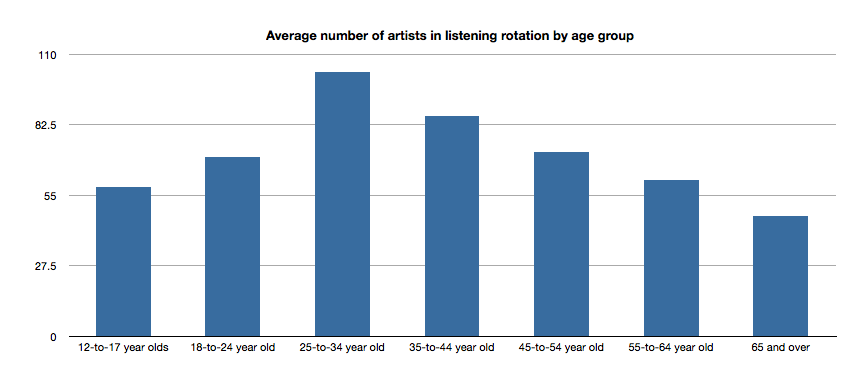
Average number of artists in listening rotation
The typical 25- to 34-year old listener has more artists in active rotation than any other age group, while the 65+ listeners have the least.
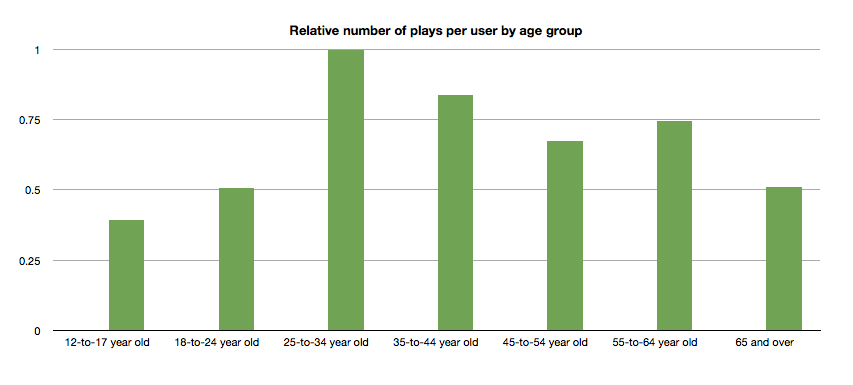
Relative number of plays per user by age group
Likewise, the typical 25- to 34-year-old listener plays more music than any other category.
Tying it all up …
This quick tour through the ages confirms our thinking that the age of a listener plays a significant role in the type of music that they listen to. We can use this information to find music that is distinctive for a particular demographic. We can also use this information to help find artists that may be acceptable to a wide range of listeners. But we should be careful to consider how popularity bias may affect our view of the world. And perhaps most important of all, people don’t like music from the 70s or 80s so much.
Gender Specific Listening
Posted by Paul in data, Music, music information retrieval, recommendation, research, The Echo Nest, zero ui on February 10, 2014
One of the challenges faced by a music streaming service is to figure out what music to play for the brand-new listener. The first listening experience of a new listener can be critical to gaining that listener as a long time subscriber. However, figuring out what to play for that new listener is very difficult because often there’s absolutely no data available about what kind of music that listener likes. Some music services will interview the new listener to get an idea of their music tastes.
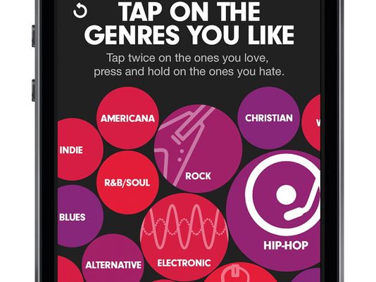
Selecting your favorite genres is part of the nifty user interview for Beat’s music
However, we’ve seen that for many listeners, especially the casual and indifferent listeners, this type of enrollment may be too complicated. Some listeners don’t know or care about the differences between Blues, R&B and Americana and thus won’t be able to tell you which they prefer. A listener whose only experience in starting a listening session is to turn on the radio may not be ready for a multi-screen interview about their music taste.
So what can a music service play for a listener when they have absolutely no data about that listener? A good place to start is to play music by the most popular artists. Given no other data, playing what’s popular is better than nothing. But perhaps we can do better than that. The key is in looking at the little bit of data that a new listener will give you.
For most music services, there’s a short user enrollment process that gets some basic info from the listener including their email address and some basic demographic information. Here’s the enrollment box for Spotify:
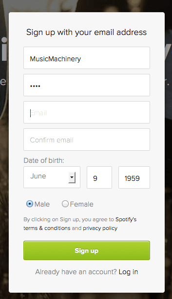
Included in this information is the date of birth and the gender of the listener. Perhaps we can use basic demographic data to generate a slightly more refined set of artists. For starters, lets consider gender. Let’s try to answer the question: If we know that a listener is male or female does that increase our understanding of what kind of music they might like? Let’s take a look.
Exploring Gender Differences in Listening
Do men listen to different music than women do? Anecdotally, we can think of lots of examples that point to yes – it seems like more of One Direction’s fans are female, while more heavy metal fans are male, but lets take a look at some data to see if this is really the case.
The Data – For this study, I looked at the recent listening of about 200 thousand randomly selected listeners that have self-identified as either male or female. From this set of listeners, I tallied up the number of male and female listeners for each artist and then simply ranked the artists in order or listeners. Here’s a quick look at the top 5 artists by gender.
Top 5 artists by gender
| Rank | All | Male | Female |
|---|---|---|---|
| 1 | Rihanna | Eminem | Rihanna |
| 2 | Bruno Mars | Daft Punk | Bruno Mars |
| 3 | Eminem | Jay-Z | Beyoncé |
| 4 | Katy Perry | Bruno Mars | Katy Perry |
| 5 | Justin Timberlake | Drake | P!nk |
Among the top 5 we see that the Male and Female listeners only share one artist in common:Bruno Mars. This trend continues as we look at the top 40 artists. Comparing lists by eye can be a bit difficult, so I created a slopegraph visualization to make it easier to compare. Click on this image to see the whole slopegraph:

click for full chart
Looking at the top 40 charts artists we see that more than a quarter of the artists are gender specific. Artists that top the female listener chart but are missing on the male listener chart include: Justin Bieber, Demi Lovato, Shakira, Britney Spears, One Direction, Christina Aguilera, Ke$ha, Ciara, Jennifer Lopez, Avril Lavigne and Nicki Minaj. Conversely, artists that top the male listener chart but are missing on the top 40 female listener chart include: Bob Marley, Kendrick Lamar, Wiz Khalifa, Avicii, T.I. Queen, J.Cole, Linkin Park, Kid Cudi and 50 Cent. While some artists seem to more easily cross gender lines like Rihanna, Justin Timberlake, Lana Del Rey and Robin Thicke.
No matter what size chart we look at – whether it is the top 40, top 200 or the top 1000 artists – about 30% of artists on a gender-specific chart don’t appear on the corresponding chart for the opposite gender. Similarly, about 15% of the artists that appear on a general chart of top artists will be of low relevance to a typical listener based on these gender-listening differences.
What does this all mean? If you don’t know anything about a listener except for their gender, you can reduce the listener WTFs by 15% for a typical listener by restricting plays to artists from the gender specific charts. But perhaps even more importantly, we can use this data to improve the listening experience for a listener even if we don’t know a listener’s gender at all. Looking at the data we see that there are a number of gender-polarizing artists on any chart. These are artists that are extremely popular for one gender, but not popular at all for the other. Chances are that if you play one of these polarizing artists for a listener that you know absolutely nothing about, 50% of the time you will get it wrong. Play One Direction and 50% of the time the listener won’t like it, just because 50% of the time the listener is male. This means that we can improve the listening experience for a listener, even if we don’t know their gender by eliminating the gender skewing artists and replacing them with more gender neutral artists.
Let’s see how this would affect our charts. Here are the new Top 40 artists when we account for gender differences.
| Rank | Old Rank | Artist |
|---|---|---|
| 1 | 2 | Bruno Mars |
| 2 | 1 | Rihanna |
| 3 | 5 | Justin Timberlake |
| 4 | 4 | Katy Perry |
| 5 | 6 | Drake |
| 6 | 15 | Chris Brown |
| 7 | 3 | Eminem |
| 8 | 8 | P!nk |
| 9 | 11 | David Guetta |
| 10 | 14 | Usher |
| 11 | 17 | Maroon 5 |
| 12 | 7 | Jay-Z |
| 13 | 13 | Adele |
| 14 | 9 | Beyoncé |
| 15 | 12 | Lil Wayne |
| 16 | 23 | Lana Del Rey |
| 17 | 25 | Robin Thicke |
| 18 | 24 | Pitbull |
| 19 | 27 | The Black Eyed Peas |
| 20 | 19 | Lady Gaga |
| 21 | 20 | Michael Jackson |
| 22 | 10 | Daft Punk |
| 23 | 18 | Miley Cyrus |
| 24 | 22 | Macklemore & Ryan Lewis |
| 25 | 28 | Coldplay |
| 26 | 16 | Taylor Swift |
| 27 | 26 | Calvin Harris |
| 28 | 21 | Alicia Keys |
| 29 | 29 | Imagine Dragons |
| 30 | 30 | Britney Spears |
| 31 | 44 | Ellie Goulding |
| 32 | 31 | Kanye West |
| 33 | 42 | J. Cole |
| 34 | 41 | T.I. |
| 35 | 52 | LMFAO |
| 36 | 32 | Shakira |
| 37 | 35 | Bob Marley |
| 38 | 54 | will.i.am |
| 39 | 36 | Ke$ha |
| 40 | 39 | Wiz Khalifa |
Artists promoted to the chart due to replace gender-skewed artists are in bold. Artists that were dropped from the top 40 are:
- Avicii – skews male
- Justin Bieber – skews female
- Christina Aguilera – skews female
- One Direction – skews female
- Demi Lovato – skews female
Who are the most gender skewed artists?
The Top 40 is a fairly narrow slice of music. It is much more interesting to look at how listening can skew across a much broader range of music. Here I look at the top 1,000 artists listened to by males and the top 1,000 artists listened to by females and find the artists that have the largest change in rank as they move from the male chart to the female chart. Artists that lose the most rank are artists that skew male the most, while artists that gain the most rank skew female.
Top male-skewed artists:
artists that skew towards male fans
- Iron Maiden
- Rage Against the Machine
- Van Halen
- N.W.A
- Jimi Hendrix
- Limp Bizkit
- Wu-Tang Clan
- Xzibit
- The Who
- Moby
- Alice in Chains
- Soundgarden
- Black Sabbath
- Stone Temple Pilots
- Mobb Deep
- Queens of the Stone Age
- Ice Cube
- Kavinsky
- Audioslave
- Pantera
Top female-skewed artists:
artists that skew towards female fans
- Danity Kane
- Cody Simpson
- Hannah Montana
- Emily Osment
- Playa LImbo
- Vanessa Hudgens
- Sandoval
- Miranda Lambert
- Sugarland
- Aly & AJ
- Christina Milian
- Noel Schajris
- Maria José
- Jesse McCartney
- Bridgit Mendler
- Ashanti
- Luis Fonsi
- La Oreja de Van Gogh
- Michelle Williams
- Lindsay Lohan
Gender-skewed Genres
By looking at the genres of the most gender skewed artists we can also get a sense of which genres are most gender skewed as well. Looking at the genres of the top 1000 artists listened to by male listeners and the top 1000 artists with female listeners we identify the most skewed genres:
Genres most skewed to female listeners:
- Pop
- Dance Pop
- Contemporary Hit Radio
- Urban Contemporary
- R&B
- Hot Adult Contemporary
- Latin Pop
- Teen Pop
- Neo soul
- Latin
- Pop rock
- Contemporary country
Genres most skewed to male listeners:
- Rock
- Hip Hop
- House
- Album Rock
- Rap
- Pop Rap
- Indie Rock
- Funk Rock
- Gangster Rap
- Electro house
- Classic rock
- Nu metal
Summary
This study confirms what we expected – that there are differences in gender listening. For mainstream listening about 30% of the artists in a typical male’s listening rotation won’t be found in a typical female listening rotation and vice versa. If we happen to know a listener’s gender and nothing else, we can improve their listening experience somewhat by replacing artists that skew to the opposite gender with more neutral artists. We can even improve the listening experience for a listener that we know absolutely nothing about – not even their gender – by replacing gender-polarized artists with artists that are more accepted by both genders.
Of course when we talk about gender differences in listening, we are talking about probabilities and statistics averaged over a large number of people. Yes, the typical One Direction fan is female, but that doesn’t mean that all One Direction fans are female. We can use gender to help us improve the listening experience for a brand new user, even if we don’t know the gender of that new user. But I suspect the benefits of using gender for music scheduling is limited to helping with the cold start problem. After a new user has listened to a dozen or so songs, we’ll have a much richer picture of the type of music they listen to – and we may discover that the new male listener really does like to listen to One Direction and Justin Bieber and that new female listener is a big classic rock fan that especially likes Jimi Hendrix.
update – 2/13 – commenter AW suggested that the word ‘bias’ was too loaded a term. I agree and have changed the post replacing ‘bias’ with ‘difference’
The Zero Button Music Player
Posted by Paul in music information retrieval, playlist, recommendation, research, The Echo Nest, zero ui on January 14, 2014
Ever since the release of the Sony Walkman 35 years ago, the play button has been the primary way we interact with music. Now the play button stands as the last barrier between a listener and their music. Read on to find out how we got here and where we are going next.
 In the last 100 years, technology has played a major role in how we listen to and experience music. For instance, when I was coming of age musically, the new music technology was the Sony Walkman. With the Walkman, you could take your music with you anywhere. You were no longer tied to your living room record player to listen to your music. You no longer had to wait and hope that the DJ would play your favorite song when you were on the road. You could put your favorite songs on a tape and bring them with you and listen to them whenever you wanted to no matter where your were. The Sony Walkman really changed how we listened to music. It popularized the cassette format, which opened the door to casual music sharing by music fans. Music fans began creating mix tapes and sharing music with their friends. The playlist was reborn, music listening changed. All because of that one device.
 We are once again in the middle of music+technology revolution. It started a dozen years ago with the first iPod and it continues now with devices like the iPhone combined with a music subscription service like Spotify, Rdio, Rhapsody or Deezer. Today, a music listener armed with an iPhone and a ten dollar-a-month music subscription is a couple of taps away from being able to listen to almost any song that has ever been recorded. All of this music choice is great for the music listener, but of course it brings its own problems. When I was listening to music on my Sony Walkman, I had 20 songs to choose from, but now I have millions of songs to choose from. What should I listen to next? The choices are overwhelming. The folks that run music subscription services realize that all of this choice for their listeners can be problematic. That’s why they are all working hard to add radio features like Rdio’s You.FM Personalized Radio. Personalized Radio simplifies the listening experience – instead of having to pick every song to play, the listener only needs to select one or two songs or artists and they will be presented with an endless mix of music that fits well with initial seeds.
Helping listeners pick music is especially important when you consider that not all music listeners are alike, and that most listeners are, at best, only casual music fans. A study conducted in 2003 and again in 2006 by Emap (A UK-based Advertising agency), summarized here by David Jennings, identified four main types of music listeners. Jennings describes these four main listening types as:
-
Savants – for whom everything in life is tied up with music
-
Enthusiasts – Music is a key part of life but is balanced with other interests
-
Casuals – Music plays a welcoming role, but other things are far more important
-
Indifferents – Would not lose much sleep if music ceased to exist.
These four listener categories are an interesting way to organize music listeners, but of course, real life isn’t so cut and dried. Listener categories change as life circumstances change (have a baby and you’ll likely become a much more casual music listener) and can even change based on context (a casual listener preparing for a long road-trip may act like a savant for a few days while she builds her perfect road-trip playlist).
In 2006, the distribution of people across these 4 categories was as follows:
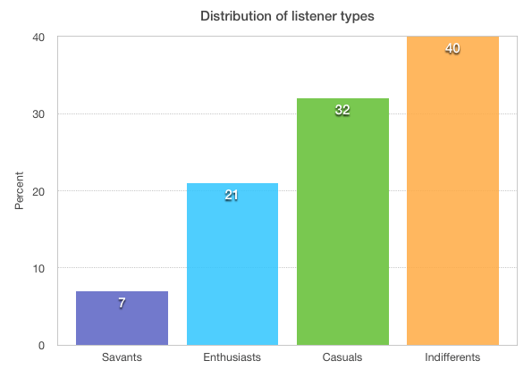
This chart says a lot about the music world and why it works the way it does. For instance, it gives us a guide as to how much different segments of the listening world are willing to pay for music in a year. On the chart below, I’ve added my estimate of the amount of money each listener type will spend on music in a year.

Savants will spend a thousand dollars or more on vinyl, concerts, and music subscriptions. Enthusiasts will spend $100 a year on a music subscription or, perhaps, purchase a couple of new tracks per week. Casuals will spend $10 a year (maybe splurge and buy that new Beyoncé album), while Indifferents will spend nothing on music. This is why music services like Spotify and Rdio have been exploring the Fremium model. If they want to enroll the 72% of people who are Casual or Indifferent music listeners, they need a product that costs much less than the $100 a year Enthusiasts are willing to pay.
However, price isn’t the only challenge music services face in attracting the Casuals and the Indifferents. Different types of listeners have a different tolerance around the amount of time and effort it takes to play music that they want to listen to.
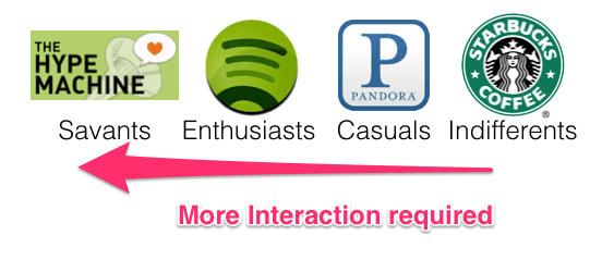
A music Savant – someone who lives, eats and breathes music – is happy spending hours a day poring through music blogs, forums and review sites to find new music, while the Indifferent music listener may not even make the simplest of efforts like turning the radio on or switching to a new station if they don’t like the current song. A simple metric for the time and effort spent is Interactions Per Listening Session. In this chart, I’ve added my estimate of the number of interactions, on average, a listener of a given type will tolerate to create a listening session.
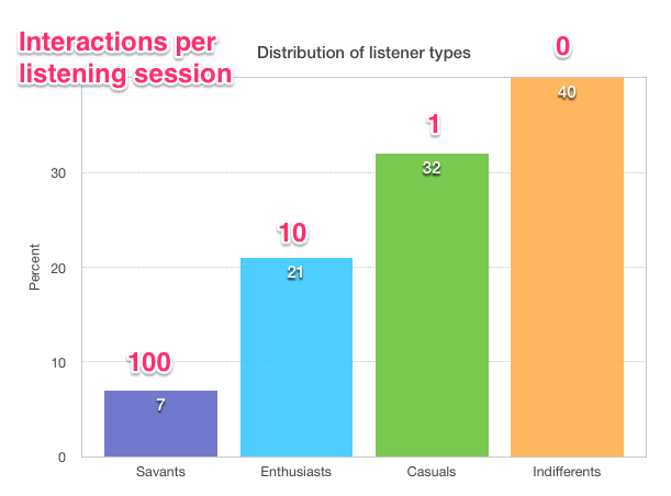
Interactions per Listening Session is an indication of how many times the listener controls their music player for a listening session. That music Savant may carefully handpick each song going into a playlist after reading a few music blogs and reviews about an artist on The Hype Machine, checking out the artist bio and previewing a few tracks. The music Enthusiast may grab a few top songs from a handful of their favorite artists to build a Spotify playlist. The casual listener may fire up Pandora, select an artist station and click play, while the Indifferent music listener may passively listen to the music that is playing on the radio or in the background at the local Starbucks.
The above chart shows why a music service like Pandora has been so successful. With its simple interface, Pandora is able to better engage the Casual listeners who don’t want to spend time organizing their listening session. A Pandora listener need only pick a station, and Pandora does all the work from there. This is why music subscription services hoping to attract more users are working hard to add Pandora-like features. In order to make their service appeal to the Casuals, they need to make it incredibly easy to have a good listening experience.
But what about those Indifferents? If 40% of people are indifferent to music, is this a lost market for music services? Is it impossible to reach people who can’t even be bothered to queue up some music on Pandora? I don’t think so. Over the last 75 years, terrestrial radio has shown that even the most indifferent music fan can be coaxed into simple, “lean back” listening. Even with all of the media distractions in the world today, 92% of Americans age 12 or older listen to the radio at least weekly, much the same as it was back in 2003 (94%).
So what does it take to capture the ears of Indifferents? First, we have to drive the out-of-pocket costs to the listener to zero. This is already being done via the Freemium model – Ad supported Internet radio (non-on-demand) is becoming the standard entry point for music services. Next, and perhaps more difficult, we have to drive the number of interactions required to listen to music to zero.
Thus my current project – Zero UI – building a music player that minimizes the interactions necessary to get good music to play – a music player that can capture the attention of even the musically indifferent.
Implicit signals and context
Perhaps the biggest challenge in creating a Zero UI music player is how to get enough information about the listener to make good music choices. If a Casual or Indifferent listener can’t be bothered to explicitly tell us what kind of music they like, we have to try to figure it out based upon implicit signals. Luckily, a listener gives us all kinds of implicit signals that we can use to understand their music taste. Every time a listener adjusts the volume on the player, every time they skip a song, every time they search for an artist, or whenever they abandon a listening session, they are telling us a little bit about their music taste. In addition to the information we can glean from a listener’s implicit actions, there’s another source of data that we can use to help us understand a music listener. That’s the listener’s music listening device – i.e. their phone.

The mobile phone is now and will continue to be the primary way for people to interact with and experience music. My phone is connected to a music service with 25 million songs. It ‘knows’ in great detail what music I like and what I don’t like. It knows some basic info about me such as my age and sex. It knows where I am, and what I am doing – whether I’m working, driving, doing chores or just waking up. It knows my context – the time of day, the day of the week, today’s weather, and my schedule. It knows that I’m late for my upcoming lunch meeting and it even might even know the favorite music of the people I’m having lunch with.
Current music interfaces use very little of the extra context provided by the phone to aid in music exploration and discovery. In the Zero UI project, I’ll explore how all of this contextual information provided by the latest devices (and near future devices) can be incorporated into the music listening experience to help music listeners organize, explore, discover and manage their music listening. The goal is to create a music player that knows the best next song to play for you given your current context. No button pressing required.
There are lots of really interesting areas to explore:
-
Can we glean enough signal from the set of minimal listener inputs?
-
Which context types (user activity, location, time-of-day, etc.) are most important for scheduling music? Will we suffer from the curse of dimensionality with too many contexts?
-
What user demographic info is most useful for avoiding the cold start problem (age, sex, zip code)?
-
How can existing social data (Facebook likes, Twitter follows, social tags, existing playlists) be used to improve the listening experience?
-
How can we use information from new wearable devices such as the Jawbone’s Up, the Fitbit, and the Pebble Smart Watch to establish context?
-
How do we balance knowing enough about a listener to give them good music playlists and knowing so much about a listener that they are creeped out about their ‘stalker music player’?
Over the next few months I’ll be making regular posts about Zero-UI. I’ll share ideas, prototypes and maybe even some code. Feel free to follow along.
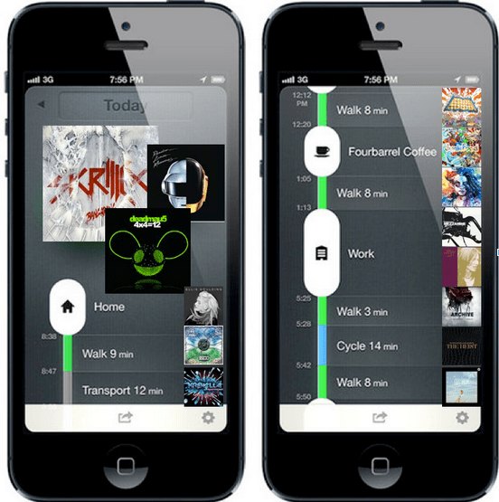
Conceptual zero-ui player that maps music listening onto user activity (as tracked by moves-app )
How to process a million songs in 20 minutes
The recently released Million Song Dataset (MSD), a collaborative project between The Echo Nest and Columbia’s LabROSA is a fantastic resource for music researchers. It contains detailed acoustic and contextual data for a million songs. However, getting started with the dataset can be a bit daunting. First of all, the dataset is huge (around 300 gb) which is more than most people want to download. Second, it is such a big dataset that processing it in a traditional fashion, one track at a time, is going to take a long time. Even if you can process a track in 100 milliseconds, it is still going to take over a day to process all of the tracks in the dataset. Luckily there are some techniques such as Map/Reduce that make processing big data scalable over multiple CPUs. In this post I shall describe how we can use Amazon’s Elastic Map Reduce to easily process the million song dataset.
The Problem

From 'Creating Music by Listening' by Tristan Jehan
For this first experiment in processing the million song data set I want to do something fairly simple and yet still interesting. One easy calculation is to determine each song’s density – where the density is defined as the average number of notes or atomic sounds (called segments) per second in a song. To calculate the density we just divide the number of segments in a song by the song’s duration. The set of segments for a track is already calculated in the MSD. An onset detector is used to identify atomic units of sound such as individual notes, chords, drum sounds, etc. Each segment represents a rich and complex and usually short polyphonic sound. In the above graph the audio signal (in blue) is divided into about 18 segments (marked by the red lines). The resulting segments vary in duration. We should expect that high density songs will have lots of activity (as an Emperor once said “too many notes”), while low density songs won’t have very much going on. For this experiment I’ll calculate the density of all 1 million songs and find the most dense and the least dense songs.
MapReduce
A traditional approach to processing a set of tracks would be to iterate through each track, process the track, and report the result. This approach, although simple, will not scale very well as the number of tracks or the complexity of the per track calculation increases. Luckily, a number of scalable programming models have emerged in the last decade to make tackling this type of problem more tractable. One such approach is MapReduce.
MapReduce is a programming model developed by researchers at Google for processing and generating large data sets. With MapReduce you specify a map function that processes a key/value pair to generate a set of intermediate key/value pairs, and a reduce function that merges all intermediate values associated with the same intermediate key. There are a number of implementations of MapReduce including the popular open sourced Hadoop and Amazon’s Elastic MapReduce.
There’s a nifty MapReduce Python library developed by the folks at Yelp called mrjob. With mrjob you can write a MapReduce task in Python and run it as a standalone app while you test and debug it. When your mrjob is ready, you can then launch it on a Hadoop cluster (if you have one), or run the job on 10s or even 100s of CPUs using Amazon’s Elastic MapReduce. Writing an mrjob MapReduce task couldn’t be easier. Here’s the classic word counter example written with mrjob:
from mrjob.job import MRJob

class MRWordCounter(MRJob):
    def mapper(self, key, line):
        for word in line.split():
            yield word, 1

    def reducer(self, word, occurrences):
        yield word, sum(occurrences)

if __name__ == '__main__':
    MRWordCounter.run()
The input is presented to the mapper function, one line at a time. The mapper breaks the line into a set of words and emits a word count of 1 for each word that it finds. The reducer is called with a list of the emitted counts for each word, it sums up the counts and emits them.
When you run your job in standalone mode, it runs in a single thread, but when you run it on Hadoop or Amazon (which you can do by adding a few command-line switches), the job is spread out over all of the available CPUs.
MapReduce job to calculate density
We can calculate the density of each track with this very simple mrjob – in fact, we don’t even need a reducer step:
class MRDensity(MRJob):
    """ A  map-reduce job that calculates the density """

    def mapper(self, _, line):
        """ The mapper loads a track and yields its density """
        t = track.load_track(line)
        if t:
            if t['tempo'] > 0:
                density = len(t['segments']) / t['duration']
                yield (t['artist_name'], t['title'], t['song_id']), density
(see the full code on github)
The mapper loads a line and parses it into a track dictionary (more on this in a bit), and if we have a good track that has a tempo then we calculate the density by dividing the number of segments by the song’s duration.
Parsing the Million Song Dataset
We want to be able to process the MSD with code running on Amazon’s Elastic MapReduce. Since the easiest way to get data to Elastic MapReduce is via Amazon’s Simple Storage Service (S3), we’ve loaded the entire MSD into a single S3 bucket at http://tbmmsd.s3.amazonaws.com/. (The ‘tbm’ stands for Thierry Bertin-Mahieux, the man behind the MSD). This bucket contains around 300 files each with data on about 3,000 tracks. Each file is formatted with one track per line following the format described in the MSD field list. You can see a small subset of this data for just 20 tracks in this file on github: tiny.dat. I’ve written track.py that will parse this track data and return a dictionary containing all the data.
You are welcome to use this S3 version of the MSD for your Elastic MapReduce experiments. But note that we are making the S3 bucket containing the MSD available as an experiment. If you run your MapReduce jobs in the “US Standard Region” of Amazon, it should cost us little or no money to make this S3 data available. If you want to download the MSD, please don’t download it from the S3 bucket, instead go to one of the other sources of MSD data such as Infochimps. We’ll keep the S3 MSD data live as long as people don’t abuse it.
Running the Density MapReduce job
You can run the density MapReduce job on a local file to make sure that it works:
% python density.py tiny.dat
This creates output like this:
["Planet P Project", "Pink World", "SOIAZJW12AB01853F1"]	3.3800521773317689
["Gleave", "Come With Me", "SOKBZHG12A81C21426"]	7.0173630509232234
["Chokebore", "Popular Modern Themes", "SOGVJUR12A8C13485C"]	2.7012807851495166
["Casual", "I Didn't Mean To", "SOMZWCG12A8C13C480"]	4.4351713380683542
["Minni the Moocher", "Rosi_ das M\u00e4dchen aus dem Chat", "SODFMEL12AC4689D8C"]	3.7249476012698159
["Rated R", "Keepin It Real (Skit)", "SOMJBYD12A6D4F8557"]	4.1905674943168156
["F.L.Y. (Fast Life Yungstaz)", "Bands", "SOYKDDB12AB017EA7A"]	4.2953929132587785
Where each ‘yield’ from the mapper is represented by a single line in the output, showing the track ID info and the calculated density.
Running on Amazon’s Elastic MapReduce
When you are ready to run the job on a million songs, you can run it the on Elastic Map Reduce. First you will need to set up your AWS system. To get setup for Elastic MapReduce follow these steps:
- create an Amazon Web Services account: <http://aws.amazon.com/>
- sign up for Elastic MapReduce: <http://aws.amazon.com/elasticmapreduce/>
- Get your access and secret keys (go to <http://aws.amazon.com/account/> and click on “Security Credentials”)
- Set the environment variables $AWS_ACCESS_KEY_ID and $AWS_SECRET_ACCESS_KEY accordingly for mrjob.
Once you’ve set things up, you can run your job on Amazon using the entire MSD as input by adding a few command switches like so:
% python density.py --num-ec2-instances 100 --python-archive t.tar.gz -r emr 's3://tbmmsd/*.tsv.*' > out.dat
The ‘-r emr’ says to run the job on Elastic Map Reduce, and the ‘–num-ec2-instances 100’ says to run the job on 100 small EC2 instances. A small instance currently costs about ten cents an hour billed in one hour increments, so this job will cost about $10 to run if it finishes in less than an hour, and in fact this job takes about 20 minutes to run. If you run it on only 10 instances it will cost 1 or 2 dollars. Note that the t.tar.gz file simply contains any supporting python code needed to run the job. In this case it contains the file track.py. See the mrjob docs for all the details on running your job on EC2.
The Results
The output of this job is a million calculated densities, one for each track in the MSD. We can sort this data to find the most and least dense tracks in the dataset. Here are some high density examples:
Ichigo Ichie by Ryuji Takeuchi has a density of 9.2 segments/second

Ichigo Ichie by Ryuji Takeuchi
129 by Strojovna 07 has a density of 9.2 segments/second

129 by Strojovna 07
The Feeding Circle by Makaton with a density of 9.1 segments per segment

The Feeding Circle by Makaton
Indeed, these pass the audio test, they are indeed high density tracks. Now lets look at some of the lowest density tracks.
Deviation by Biosphere with a density of .014 segments per second

Deviation by Biosphere
The Wire IV by Alvin Lucier with a density of 0.014 segments per second

The Wire IV by Alvin Lucier
improvisiation_122904b by Richard Chartier with a density of .02 segments per second

improvisation by Richard Chartier
Wrapping up
The ‘density’ MapReduce task is about as simple a task for processing the MSD that you’ll find. Consider this the ‘hello, world’ of the MSD. Over the next few weeks, I’ll be creating some more complex and hopefully interesting tasks that show some of the really interesting knowledge about music that can be gleaned from the MSD.
(Thanks to Thierry Bertin-Mahieux for his work in creating the MSD and setting up the S3 buckets. Thanks to 7Digital for providing the audio samples)
How do you discover music?
Posted by Paul in Music, recommendation, research on August 18, 2011
I’m interested in learning more about how people are discovering new music. I hope that you will spend 2 mins and take this 3 question poll. I’ll publish the results in a few weeks.
How do you spell ‘Britney Spears’?
Posted by Paul in code, data, Music, music information retrieval, research, The Echo Nest on July 28, 2011
I’ve been under the weather for the last couple of weeks, which has prevented me from doing most things, including blogging. Luckily, I had a blog post sitting in my drafts folder almost ready to go. I spent a bit of time today finishing it up, and so here it is. A look at the fascinating world of spelling correction for artist names.
 In today’s digital music world, you will often look for music by typing an artist name into a search box of your favorite music app. However this becomes a problem if you don’t know how to spell the name of the artist you are looking for. This is probably not much of a problem if you are looking for U2, but it most definitely is a problem if you are looking for Röyksopp, Jamiroquai or Britney Spears. To help solve this problem, we can try to identify common misspellings for artists and use these misspellings to help steer you to the artists that you are looking for.
A spelling corrector in 21 lines of code
A good place for us to start is a post by Peter Norvig (Director of Research at Google) called ‘How to write a spelling corrector‘ which presents a fully operational spelling corrector in 21 lines of Python. (It is a phenomenal bit of code, worth the time studying it). At the core of Peter’s algorithm is the concept of the edit distance which is a way to represent the similarity of two strings by calculating the number of operations (inserts, deletes, replacements and transpositions) needed to transform one string into the other. Peter cites literature that suggests that 80 to 95% of spelling errors are within an edit distance of 1 (meaning that most misspellings are just one insert, delete, replacement or transposition away from the correct word). Not being satisfied with that accuracy, Peter’s algorithm considers all words that are within an edit distance of 2 as candidates for his spelling corrector. For Peter’s small test case (he wrote his system on a plane so he didn’t have lots of data nearby), his corrector covered 98.9% of his test cases.
Spell checking Britney
A few years ago, the smart folks at Google posted a list of Britney Spears spelling corrections that shows nearly 600 variants on Ms. Spears name collected in three months of Google searches. Perusing the list, you’ll find all sorts of interesting variations such as ‘birtheny spears’ , ‘brinsley spears’ and ‘britain spears’. I suspect that some these queries (like ‘Brandi Spears’) may actually not be for the pop artist. One curiosity in the list is that although there are 600 variations on the spelling of ‘Britney’ there is exactly one way that ‘spears’ is spelled. There’s no ‘speers’ or ‘spheres’, or ‘britany’s beers’ on this list.
One thing I did notice about Google’s list of Britneys is that there are many variations that seem to be further away from the correct spelling than an edit distance of two at the core of Peter’s algorithm. This means that if you give these variants to Peter’s spelling corrector, it won’t find the proper spelling. Being an empiricist I tried it and found that of the 593 variants of ‘Britney Spears’, 200 were not within an edit distance of two of the proper spelling and would not be correctable. This is not too surprising. Names are traditionally hard to spell, there are many alternative spellings for the name ‘Britney’ that are real names, and many people searching for music artists for the first time may have only heard the name pronounced and have never seen it in its written form.
Making it better with an artist-oriented spell checker
A 33% miss rate for a popular artist’s name seems a bit high, so I thought I’d see if I could improve on this. I have one big advantage that Peter didn’t. I work for a music data company so I can be pretty confident that all the search queries that I see are going to be related to music. Restricting the possible vocabulary to just artist names makes things a whole lot easier. The algorithm couldn’t be simpler. Collect the names of the top 100K most popular artists. For each artist name query, find the artist name with the smallest edit distance to the query and return that name as the best candidate match. This algorithm will let us find the closest matching artist even if it is has an edit distance of more than 2 as we see in Peter’s algorithm. When I run this against the 593 Britney Spears misspellings, I only get one mismatch – ‘brandi spears’ is closer to the artist ‘burning spear’ than it is to ‘Britney Spears’. Considering the naive implementation, the algorithm is fairly fast (40 ms per query on my 2.5 year old laptop, in python).
Looking at spelling variations
With this artist-oriented spelling checker in hand, I decided to take a look at some real artist queries to see what interesting things I could find buried within. I gathered some artist name search queries from the Echo Nest API logs and looked for some interesting patterns (since I’m doing this at home over the weekend, I only looked at the most recent logs which consists of only about 2 million artist name queries).
Artists with most spelling variations
Not surprisingly, very popular artists are the most frequently misspelled. It seems that just about every permutation has been made in an attempt to spell these artists.
- Michael Jackson – Variations: michael jackson, micheal jackson, michel jackson, mickael jackson, mickal jackson, michael jacson, mihceal jackson, mickeljackson, michel jakson, micheal jaskcon, michal jackson, michael jackson by pbtone, mical jachson, micahle jackson, machael jackson, muickael jackson, mikael jackson, miechle jackson, mickel jackson, mickeal jackson, michkeal jackson, michele jakson, micheal jaskson, micheal jasckson, micheal jakson, micheal jackston, micheal jackson just beat, micheal jackson, michal jakson, michaeljackson, michael joseph jackson, michael jayston, michael jakson, michael jackson mania!, michael jackson and friends, michael jackaon, micael jackson, machel jackson, jichael mackson
- Justin Bieber – Variations: justin bieber, justin beiber, i just got bieber’ed by, justin biber, justin bieber baby, justin beber, justin bebbier, justin beaber, justien beiber, sjustin beiber, justinbieber, justin_bieber, justin. bieber, justin bierber, justin bieber<3 4 ever<3, justin bieber x mstrkrft, justin bieber x, justin bieber and selens gomaz, justin bieber and rascal flats, justin bibar, justin bever, justin beiber baby, justin beeber, justin bebber, justin bebar, justien berbier, justen bever, justebibar, jsustin bieber, jastin bieber, jastin beiber, jasten biber, jasten beber songs, gestin bieber, eiine mainie justin bieber, baby justin bieber,
- Red Hot Chili Peppers – Variations: red hot chilli peppers, the red hot chili peppers, red hot chilli pipers, red hot chilli pepers, red hot chili, red hot chilly peppers, red hot chili pepers, hot red chili pepers, red hot chilli peppears, redhotchillipeppers, redhotchilipeppers, redhotchilipepers, redhot chili peppers, redhot chili pepers, red not chili peppers, red hot chily papers, red hot chilli peppers greatest hits, red hot chilli pepper, red hot chilli peepers, red hot chilli pappers, red hot chili pepper, red hot chile peppers
- Mumford and Sons – Variations: mumford and sons, mumford and sons cave, mumford and son, munford and sons, mummford and sons, mumford son, momford and sons, modfod and sons, munfordandsons, munford and son, mumfrund and sons, mumfors and sons, mumford sons, mumford ans sons, mumford and sonns, mumford and songs, mumford and sona, mumford and, mumford &sons, mumfird and sons, mumfadeleord and sons
- Katy Perry – Even an artist with a seemingly very simple name like Katy Perry has numerous variations: katy perry, katie perry, kate perry, kathy perry, katy perry ft.kanye west, katty perry, katy perry i kissed a girl, peacock katy perry, katyperry, katey parey, kety perry, kety peliy, katy pwrry, katy perry-firework, katy perry x, katy perry, katy perris, katy parry, kati perry, kathy pery, katey perry, katey perey, katey peliy, kata perry, kaity perry
Some other most frequently misspelled artists:
- Britney Spears
- Linkin Park
- Arctic Monkeys
- Katy Perry
- Guns N’ Roses
- Nicki Minaj
- Muse
- Weezer
- U2
- Oasis
- Moby
- Flyleaf
- Seether
- byran adams – ryan adams
- Underworld – Uverworld
Reidentification of artists and genres in the KDD cup data
Posted by Paul in data, recommendation, research on June 21, 2011
Back in February I wrote a post about the KDD Cup ( an annual Data Mining and Knowledge Discovery competition), asking whether this year’s cup was really music recommendation since all the data identifying the music had been anonymized. The post received a number of really interesting comments about the nature of recommendation and whether or not context and content was really necessary for music recommendation, or was user behavior all you really needed. A few commenters suggested that it might be possible de-anonymize the data using a constraint propagation technique.
 Many voiced an opinion that such de-anonymizing of the data to expose user listening habits would indeed be unethical. Malcolm Slaney, the researcher at Yahoo! who prepared the dataset offered the plea:
If you do de-anonymize the data please don’t tell anybody. We’ll NEVER be able to release data again.
As far as I know, no one has de-anonymized the KDD Cup dataset, however, researcher Matthew J. H. Rattigan of The University of Massachusetts at Amherst has done the next best thing. He has published a paper called Reidentification of artists and genres the KDD cup that shows that by analyzing at the relational structures within the dataset it is possible to identify the artists, albums, tracks and genres that are used in the anonymized dataset. Here’s an excerpt from the paper that gives an intuitive description of the approach:
For example, consider Artist 197656 from the Track 1 data. This artist has eight albums described by different combinations of ten genres. Each album is associated with several tracks, with track counts ranging from 1 to 69. We make the assumption that these albums and tracks were sampled without replacement from the discography of some real artist on the Yahoo! Music website. Furthermore, we assume that the connections between genres and albums are not sampled; that is, if an album in the KDD Cup dataset is attached to three genres, its real-world counterpart has exactly three genres (or “Categories”, as they are known on the Yahoo! Music site).
Under the above assumptions, we can compare the unlabeled KDD Cup artist with real-world Yahoo! Music artists in order to find a suitable match. The band Fischer Z, for example, is an unsuitable match, as their online discography only contains seven albums. An artist such as Meatloaf certainly has enough albums (56) to be a match, but none of those albums contain more than 31 tracks. The entry for Elvis Presley contains 109 albums, 17 of which boast 69 or more tracks; however, there is no consistent assignment of genres that satisfies our assumptions. The band Tool, however, is compatible with Artist 197656. The Tool discography contains 19 albums containing between 0 and 69 tracks. These albums are described by exactly 10 genres, which can be assigned to the unlabeled KDD Cup genres in a consistent manner. Furthermore, the match is unique: of the 134k artists in our labeled dataset, Tool is the only suitable match for Artist 197656.
Of course it is impossible for Matthew to evaluate his results directly, but he did create a number of synthetic, anonymized datasets draw from Yahoo and was able to demonstrate very high accuracy for the top artists and a 62% overall accuracy.
The motivation for this type of work is not to turn the KDD cup dataset into something that music recommendation researchers could use, but instead is to get a better understanding of data privacy issues. By understanding how large datasets can be de-anonymized, it will be easier for researchers in the future to create datasets that won’t be easily yield their hidden secrets. The paper is an interesting read – so since you are done doing all of your reviews for RecSys and ISMIR, go ahead and give it a read: https://www.cs.umass.edu/publication/docs/2011/UM-CS-2011-021.pdf. Thanks to @ocelma for the tip.
catfish smooth
Posted by Paul in data, Music, recommendation, research on January 20, 2011
Kurt Jacobson is a recent additions to the staff here at The Echo Nest. Kurt has built a music exploration site called catfish smooth that allows you to explore the connections between artists. Kurt describes it as: all about connections between music artists. In a sense, it is a music artist recommendation system but more. For each artist, you will see the type of “similar artist” recommendations to which you are accustomed – we use last.fm and The Echo Nest to get these. But you will also see some other inter-artist connections catfish has discovered from the web of linked data. These include things like “artists that are also English Male Singers” or “artists that are also Converts To Islam” or “artists that are also People From St.Louis, Missouri”. And, hopefully, you’ll get some media for each artist so you can have a listen.
It’s a really interesting way to explore the music space, allowing you to stumble upon new artists based on a wide range of parameters.

For example take a look at the many categories and connections catfish smooth exposes for James Brown.

Kurt is currently conducting a usability survey for catfish smooth, so take a minute to kick the tires and then help Kurt finish his PhD and take the survey.
SongCards – an untapped app
I saw this interesting video from IDEO for c60 – an RFID-based interface that ‘reintroduces physicality to music, something lost with digitization and the move to the cloud.’
This video got me excited, because it is the hardware piece of an idea that my friend Steve Green and I had called ‘SongCards’ while working at Sun Labs a few years ago. We pitched SongCards to Sun’s management (Sun was big into RFID at the time so it seemed like a good fit), but Sun didn’t bite – they decided to go buy MySql instead. And so this concept has been gathering digital dust in a text file on my laptop. The c60 video has inspired me to dust it off and post i here. I think there are some good ideas embedded in the concept. Perhaps the folks at IDEO will incorporate some into the c60, or maybe Eliot will add this idea to his Untapped Apps portfolio on Evolver.fm.
Here’s the concept in all its glory:
Observations
- Many people have a physical connection with their music. These people like to organize, display and interact with their music via the containers (album covers, cd cases).
- Music is a highly social medium. People enjoy sharing music with others. People learn about new music from others in their social circle.
- The location where music is stored will likely switch from devices managed by the listener to devices managed by a music service. In the future, a music purchaser will purchase the right to listen to a particular song, while the actual music data will remain managed by the music service.
- Digital music lacks much of the interesting metadata that previous generations of music listeners enjoyed – lyrics, photos of the performers, song credits. The experience of reading the liner notes while listening to a new album has been lost in this new generation of digital music.Music is collectable. People take pride in amassing large collections of music and like to be able to exhibit their collection to others.
The Problem
The digital music revolution and the inevitable move of our music from our CD racks, iPods and computers, to the back room at Yahoo, Apple, or Google will make it convenient for people to listen to music in all sorts of new ways, however at the same time it will eliminate many of the interactions people have had with the music. People can’t interact with the albums, read the liner notes, display their collection. They can’t trade songs with their friends. There is no way to show off a music collection beyond saying “I have 2,025 songs on my iPod”. Album art is a dying art.
weMusic collecting is not just about the music, it also is about the things that surround the music. Digital music has stripped away all of the packaging, and at the same time has stripped away a big part of the music collecting experience. We want to change that.
The Idea
 Imagine if you could buy music like you buy collectable trading cards such as Magic the Gathering, or Pokemon cards. One could buy a pack of cards at the local 7-11 for a few dollars. The cards could be organized by genre. You could buy a pack of ‘boy-band’, ‘alternative-grunge’, ‘brit-pop’, ‘British invasion ‘, ‘drum and bass’ etc. Each pack would contain 5 or 10 cards draw from the genre of the pack. Each card would have all of the traditional liner note metadata: lyrics, album art, artist bios. Also associated with each card would be a unique ID that can be read by an electronic reader that would identify the unique instance of the card and the song/performance that the card represents. The new owner of the card would add the song to their personal collection by just presenting it to any of the owner’s music players (presumably they are connected to the music server run by the music service provider). Once this is done, the user can access and play the song at any time on any of their music devices.
A package of music cards can be packaged in the same way as other trading cards are packaged. Typically in each pack there are one or two ‘special’ cards that are highly desirable. For music cards these would be the highly desirable ‘hit cards’. The bulk of the cards in a deck could be made up of lesser known, or less popular bands. For instance a ‘British invasion’ card set may contain ‘hey jude’ as the special card, and a few lesser known Beatles songs, and few songs by “the who” and perhaps some by “the monkees” and other songs by bands of that era. This method of packing music would allow for serendipitous discovery of music since you would never know what songs you would get in the pack. It would also encourage music trading, since you could trade your duplicate songs with other music collectors.
Trading – since the cards represent a song by a digital id, trading a song is as simple as giving the card to someone. As soon as the new owner of the card puts the card into one of their music players the transfer of ownership would occur, the song would be added to the collection of the new owner and removed from the collection of the old owner. There would be no limit to how often a song could be traded.
Some interesting properties of music cards:
- Your music collection once again has a physical presence. You can touch it, you can browse through it, you can stack it, you can show it off.
- You can easily and legally trade or sell music with your friends (or on eBay for that matter). Supply and demand economics can take hold in the music card after market (just as we’ve seen with Beanie Babies and Magic cards).Cards can be grouped in packages for sale using a number of criteria such as genre, popularity, geography, appeal to a certain demographic.
- You can make playlists by ordering your cards.
- You can make a random playlist by shuffling your cards.
- At a social gathering, cards from many people can be combined into a single uber-playlist.
- You will be potentially exposed to new music every time you buy a new pack of cards.
- You will not need to carry your cards with you when you want to listen to music (the music service knows what music you own).
- Since the music service ‘knows’ what music you own it can monitor trades and music popularity to track trend setters within a social group and target appropriate marketing at the trend setters.
- Song cards can’t be ‘ripped’ in the traditional sense, giving music companies much more control over their intellectual property.
Some interesting variations:
- The artwork on the back of a card could be one section of the album art for a whole album. You could tack the cards up on the wall to form the album art when you have the whole album.
- Some of the cards could be power cards that act as modifiers:
- ‘More Like This‘ when inserted into a playlist, plays a similar song to the previously played card. The similar song is drawn from the entire music service collection not just the songs owned by the collector.
- Genre Wild card’ – plays a random song from the genre. The similar song is drawn from the entire music service collection not just the songs owned by the collector.
- ‘Musical Journey‘ – make a musical journey between the surrounding cards. The songs on the journey are drawn from the entire music service collection not just the songs owned by the collector.
- ‘Album Card’ – it’s not just a song, it’s a whole album.
Note that I don’t think that SongCards would replace all digital music sales. It would still be possible to purchase and download a song from iTunes as one can do today. I think that SongCards would appeal to the ‘Music Collector’, while the traditional download would appeal to the ‘Music Listener’.
That’s it – SongCards – Just imagine what the world would be like if Sun had invested $800 million on SongCards instead of that open source database.
