Archive for category data
My new superpower – creating Spotify playlists from a web app
 The new Spotify Web API allows the developer to create and add tracks to a playlist on behalf of a listener. This is a pretty powerful feature, opening the door for a whole range of apps. For instance, this weekend, I added the ability to save a Roadtrip Mixtape playlist, so you can now actually take your mixtapes on the road. The code is on github if you are interested in seeing how it is done.
The Echo Nest + Spotify Sandbox
I am wearing my International Executive Music Hacker hat today. I’m writing this blog post at 5AM somewhere over the Atlantic Ocean, on my way to the Barcelona Music Hack Day, where I’ll be representing both The Echo Nest and Spotify. I’m pretty excited about the hack event – first, because it’s in freaking Barcelona, and second, because I get to talk about what’s been going on with the Spotify and Echo Nest APIs.

It has been just about 100 days since The Echo Nest and Spotify have joined forces. In that time we’ve been working hard to build the best music platform for listeners and for developers. This week we are releasing some of the very first fruits of our labors.
First up, we are releasing a new Spotify Web API.
This is a complete revamp of the Spotify Metadata API (the old version has now been deprecated). The Spotify Web API gives you access to all sorts of information about the Spotify catalog including details about artists, albums and tracks. Want to know the top tracks for an artist? There’s an API for that. Looking for high quality album art, artist images and 30 second audio previews? There are APIs for that too. Best of all, the new API includes perhaps the most requested Spotify API feature of all time With the Spotify Web API you can now create and modify playlists on behalf of authenticated users. Yes – you can now create a Spotify web app that creates playlists. (I personally requested this feature way back in 2008, here’s my begging plea for the feature in 2009).
 I’ve been using the beta version of this new API for a couple months now and I must say I am quite impressed. The API is fast, super easy to use, and provides all sorts of great data for building apps. In the past weeks I’ve had fun converting a number of my favorite apps to use the Spotify API. First there’s the Road Trip Mix Tape that lets you create a Spotify playlist of music by artists that are from the very towns you are driving through. Then there’s Music Popcorn, a visual interface for exploring genres. For the less visual, there’s the Genre Browser that gives you lots of details about the different music genres including playlists that help give you a gentle introduction to any of the thousands of Echo Nest genres. Next there’s Boil the Frog, an app that creates seamless playlists between any two artists. Finally there’s the 3D Music Maze, an app that lets you explore for music by wandering through a 3 dimensional music world.
Next up, a freshly minted Echo Nest + Spotify Sandbox — a new Spotify ID space.
 These apps are possible because of the second thing we are releasing this week – a spiffy, shiny new Spotify Rosetta Stone catalog that ensures that the Echo Nest API has the freshest, and most up-to-date view of the Spotify universe of music. For those who might be new to The Echo Nest, Project Rosetta Stone is something we’ve been working on here at the Nest for many years. The goal of Project Rosetta Stone is to solve one of the most common problems that nearly every music app developer faces. The problem is that every music service has its own set of IDs – a music subscription service like Spotify has its own artist, album and track IDs. A lyric service has its own (and very different) IDs for those same artists, albums and tracks and a concert ticketing API has yet a third set of IDs. This is quite problematic for app developers that want to build an app that combines information from multiple services. Without a common ID system, the app developer has to resort to metadata searching and matching – which is slow and quite error prone – this results in a poor app.
Project Rosetta Stone solves this problem by providing ID mappings between as many music services as we can. With this mapping you can easily translate IDs from one ID space to another. With Rosetta Stone, if you have the Spotify track ID you can get Lyricfind and/or Musixmatch IDs making it easy to use those respective APIs to retrieve lyrics for that song. You can easily map the Spotify artist ID to a Songkick or Eventful ID to get ticket and touring information from those APIs. And of course you can use the Spotify track ID to get detailed Echo Nest information about the song such as its tempo, energy, danceability, along with detailed Echo Nest artist data such as latest artist news, blog posts and similar artists.
We have had Spotify IDs in Rosetta Stone for many years, but this particular mapping has in the past been problematic for us. Spotify has a huge catalog and keeping the mapping fresh and up to date between Spotify and The Echo Nest has always been a big challenge. There’s a huge back catalog with millions of tracks to deal with plus thousands of new tracks are being added every week. The result was that there was always a bit of a lag between when updates to the Spotify catalog were reflected in the Rosetta Stone mapping. This meant that if you built a Rosetta Stone-based app you could find that The Echo Nest wouldn’t always know about a Spotify track, especially if a track was very new. The result would be a less-than-perfect app.
This week we are releasing a new Spotify ID space. Our engineers have been working hard over the last 100 days to set up all sorts of infrastructure and plumbing to ensure that we have the most up-to-date view of the Spotify catalog. No more lag between when a new track appears in Spotify and when you can get Echo Nest data. Plus, all of our APIs that take IDs as inputs will now also take Spotify IDs as input as well. If you have a Spotify artist ID you can use it with any Echo Nest artist API method. Likewise, if you have a Spotify track ID you can use it with any Echo Nest song or track API method that takes a track ID as input. This makes it **really** easy for developers to use The Echo Nest and Spotify Apps together. For example, here’s an API call that returns detailed audio properties for a Spotify track given its ID.
I’ve been having much fun using The Echo Nest API with the brand new Spotify API. I’ve already written some code that you can use. First, I wrote a Python library for Spotify called Spotipy. It’s makes it easy to write Python programs that use the new Spotify Web API, and it works well with my Echo Nest Python library called Pyen. Here’s an example of using the two libraries together:
This file contains hidden or bidirectional Unicode text that may be interpreted or compiled differently than what appears below. To review, open the file in an editor that reveals hidden Unicode characters.
Learn more about bidirectional Unicode characters
| import pyen | |
| import spotipy | |
| import sys | |
| ''' | |
| get a set of images for artists that are similar to | |
| the given seed artist | |
| ''' | |
| en = pyen.Pyen() | |
| sp = spotipy.Spotify() | |
| spids = [] | |
| response = en.get('artist/similar', name='weezer', bucket='id:spotify', limit=True) | |
| for artist in response['artists']: | |
| spids.append(artist['foreign_ids'][0]['foreign_id']) | |
| for artist in sp.artists(spids)['artists']: | |
| print artist['images'][0]['url'], artist['name'] |
I’ve also put together a number of Javascript example apps that use both APIs. These are simple apps intended to help new developers (or at least new to music apps) use the APIs together to do common things like create chillout playlists, browse through the web of similar artists, and more.
So yes, I’m pretty jazzed about this trip to Barcelona. I get to create a music hack, I get to spend a few days with some of the best music hackers in the world (The Barcelona Music Hack Day, as part of the Sonar Festival tends to attract the top music hackers). I get to spend a few days on the Mediterranean in one of the most beautiful cities in the world. Best of all, I get to talk about the new Spotify and Echo Nest developer platform and help music hackers build cool stuff on top of the newly combined platform.
I’ve put together a page that talks in detail about the new Spotify / Echo Nest platform. It has links to all of the API docs, libraries, examples, github repos, demos and details on how you can use The Echo Nest / Spotify Platform. Check it out here:
http://static.echonest.com/enspex
Keep an eye on this space for I’ll be updating it as we continue to integrate our developer APIs. There’s lots more coming, so stay tuned!
Minimizing my Karaoke pain
Rumor has it from some of the Echo Nest gang that went to Stockholm last week for new employee orientation that there is some sort of mandatory Karaoke requirement. Now for some, I’m sure this is great fun, but for others, like myself, not so much. I thought it would be best to prepare for my own mandatory Karaoke by finding some very short songs in order to minimize my time on stage. To do this I went through a database of the top Billboard songs of the last 60 years to find the shortest songs. Here are some of the top shortest popular songs of the last 60 years:
| Length(Seconds) | Artist/Title | Date |
| 76 | Anna Kendrick Cups | 2013-01-14 |
| 78 | Zac Efron What I’ve Been Looking For (Reprise) | 2006-02-13 |
| 83 | Buchanan & Goodman Santa And The Satellite (Part I) | 1957-12-25 |
| 92 | Audrey Dear Elvis (Page 1) | 1956-09-24 |
| 96 | Fats Domino Whole Lotta Loving | 1958-11-19 |
| 98 | Glee Cast Isn’t She Lovely | 2011-05-30 |
| 99 | Maurice Williams & The Zodiacs Stay | 1960-10-05 |
| 101 | Swinging Blue Jeans, The Hippy Hippy Shake | 1964-03-09 |
| 103 | Peter, Paul & Mary Settle Down (Goin’ Down That Highway) | 1963-01-21 |
| 105 | Four Tops Ain’t That Love | 1965-08-02 |
| 105 | Fats Domino Shu Rah | 1961-03-22 |
| 105 | Chuck Berry Let It Rock | 1960-02-03 |
| 107 | Lucas Gabreel & Ashley Tisdale Bop To The Top | 2006-02-13 |
| 107 | Beach Boys, The Little Deuce Coupe | 1963-08-19 |
| 107 | Clyde McPhatter Lover Please | 1962-03-05 |
| 108 | Ventures, The Hawaii Five-O | 1969-03-10 |
| 110 | Glee Cast Sing! | 2010-11-01 |
| 110 | Glee Cast It’s My Life / Confessions Part II | 2009-10-26 |
| 110 | Ricky Nelson If You Can’t Rock Me | 1963-04-22 |
So it looks like my minimum possible karaoke pain will be 76 seconds if I go with Anna Kendrick’s Cups. Certainly better than Gun’s in Roses November Rain at 8:57 seconds or Don Mclean’s American Pie at 6:49. But better yet, I can go with Hawaii Five-O . That song is not only short, but has no vocals. With that song I’m sure to be pitch perfect!
How the Autocanonizer works
Posted by Paul in code, data, events, fun, genre, hacking, music hack day, The Echo Nest on March 18, 2014
Last week at the SXSW Music Hack Championship hackathon I built The Autocanonizer. An app that tries to turn any song into a canon by playing it against a copy of itself. In this post, I explain how it works.
At the core of The Autocanonizer are three functions – (1) Build simultaneous audio streams for the two voices of the canon (2) Play them back simultaneously, (3) Supply a visualization that gives the listener an idea of what is happening under the hood. Let’s look at each of these 3 functions:
(1A) Build simultaneous audio streams – finding similar sounding beats
The goal of the Autocanonizer is to fold a song in on itself in such a way that the result still sounds musical. To do this, we use The Echo Nest analyzer and the jremix library to do much of the heavy lifting. First we use the analyzer to break the song down into beats. Each beat is associated with a timestamp, a duration, a confidence and a set of overlapping audio segments. An audio segment contains a detailed description of a single audio event in the song. It includes harmonic data (i.e. the pitch content), timbral data (the texture of the sound) and a loudness profile. Using this info we can create a Beat Distance Function (BDF) that will return a value that represents the relative distance between any two beats in the audio space. Beats that are close together in this space sound very similar, beats that are far apart sound very different. The BDF works by calculating the average distance between overlapping segments of the two beats where the distance between any two segments is a weighted combination of the euclidean distance between the pitch, timbral, loudness, duration and confidence vectors. The weights control which part of the sound takes more precedence in determining beat distance. For instance we can give more weight to the harmonic content of a beat, or the timbral quality of the beat. There’s no hard science for selecting the weights, I just picked some weights to start with and tweaked them a few times based on how well it worked. I started with the same weights that I used when creating the Infinite Jukebox (which also relies on beat similarity), but ultimately gave more weight to the harmonic component since good harmony is so important to The Autocanonizer.
(1B) Build simultaneous audio streams – building the canon
The next challenge, and perhaps biggest challenge of the whole app, is to build the canon – that is – given the Beat Distance Function, create two audio streams, one beat at a time, that sound good when played simultaneously. The first stream is easy, we’ll just play the beats in normal beat order. It’s the second stream, the canon stream that we have to worry about. The challenge: put the beats in the canon stream in an order such that (1) the beats are in a different order than the main stream, and (2) they sound good when played with the main stream.
The first thing we can try is to make each beat in the canon stream be the most similar sounding beat to the corresponding beat in the main stream. If we do that we end up with something that looks like this:
It’s a rat’s nest of connections, very little structure is evident. You can listen to what it sounds like by clicking here: Experimental Rat’s Nest version of Someone Like You (autocanonized). It’s worth a listen to get a sense of where we start from. So why does this bounce all over the place like this? There are lots of reasons: First, there’s lots of repetition in music – so if I’m in the first chorus, the most similar beat may be in the second or third chorus – both may sound very similar and it is practically a roll of the dice which one will win leading to much bouncing between the two choruses. Second – since we have to find a similar beat for every beat, even beats that have no near neighbors have to be forced into the graph which turns it into spaghetti. Finally, the underlying beat distance function relies on weights that are hard to generalize for all songs leading to more noise. The bottom line is that this simple approach leads to a chaotic and mostly non-musical canon with head-jarring transitions on the canon channel. We need to do better.
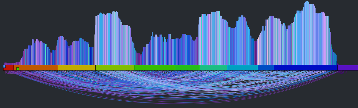
There are glimmers of musicality in this version though. Every once in a while, the canon channel will remaining on a single sequential set of beats for a little while. When this happens, it sounds much more musical. If we can make this happen more often, then we may end up with a better sounding canon. The challenge then is to find a way to identify long consecutive strands of beats that fit well with the main stream. One approach is to break down the main stream into a set of musically coherent phrases and align each of those phrases with a similar sounding coherent phrase. This will help us avoid the many head-jarring transitions that occur in the previous rat’s nest example. But how do we break a song down into coherent phrases? Luckily, it is already done for us. The Echo Nest analysis includes a breakdown of a song into sections – high level musically coherent phrases in the song – exactly what we are looking for. We can use the sections to drive the mapping. Note that breaking a song down into sections is still an open research problem – there’s no perfect algorithm for it yet, but The Echo Nest algorithm is a state-of-the-art algorithm that is probably as good as it gets. Luckily, for this task, we don’t need a perfect algorithm. In the above visualization you can see the sections. Here’s a blown up version – each of the horizontal colored rectangles represents one section:
![]()
You can see that this song has 11 sections. Our goal then is to get a sequence of beats for the canon stream that aligns well with the beats of each section. To make things at little easier to see, lets focus in on a single section. The following visualization shows the similar beat graph for a single section (section 3) in the song:
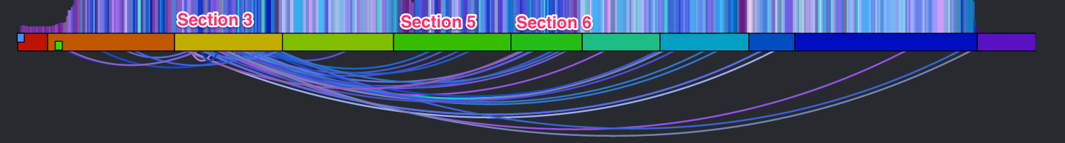
You can see bundles of edges leaving section 3 bound for section 5 and 6. We could use these bundles to find most similar sections and simply overlap these sections. However, given that sections are rarely the same length nor are they likely to be aligned to similar sounding musical events, it is unlikely that this would give a good listening experience. However, we can still use this bundling to our advantage. Remember, our goal is to find a good coherent sequence of beats for the canon stream. We can make a simplifying rule that we will select a single sequence of beats for the canon stream to align with each section. The challenge, then, is to simply pick the best sequence for each section. We can use these edge bundles to help us do this. For each beat in the main stream section we calculate the distance to its most similar sounding beat. We aggregate these counts and find the most commonly occurring distance. For example, there are 64 beats in Section 3. The most common occurring jump distance to a sibling beat is 184 beats away. There are ten beats in the section with a similar beat at this distance. We then use this most common distance of 184 to generate the canon stream for the entire section. For each beat of this section in the main stream, we add a beat in the canon stream that is 184 beats away from the main stream beat. Thus for each main stream section we find the most similar matching stream of beats for the canon stream. This visualizing shows the corresponding canon beat for each beat in the main stream.
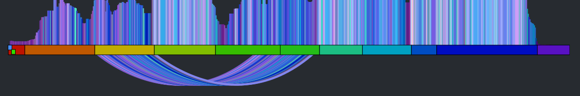
This has a number of good properties. First, the segments don’t need to be perfectly aligned with each other. Note, in the above visualization that the similar beats to section 3 span across section 5 and 6. If there are two separate chorus segments that should overlap, it is no problem if they don’t start at the exactly the same point in the chorus. The inter-beat distance will sort it all out. Second, we get good behavior even for sections that have no strong complimentary section. For instance, the second section is mostly self-similar, so this approach aligns the section with a copy of itself offset by a few beats leading to a very nice call and answer.
That’s the core mechanism of the autocanonizer – for each section in the song, find the most commonly occurring distance to a sibling beat, and then generate the canon stream by assembling beats using that most commonly occurring distance. The algorithm is not perfect. It fails badly on some songs, but for many songs it generates a really good cannon affect. The gallery has 20 or so of my favorites.
(2) Play the streams back simultaneously
When I first released my hack, to actually render the two streams as audio, I played each beat of the two streams simultaneously using the web audio API. This was the easiest thing to do, but for many songs this results in some very noticeable audio artifacts at the beat boundaries. Any time there’s an interruption in the audio stream there’s likely to be a click or a pop. For this to be a viable hack that I want to show people I really needed to get rid of those artifacts. To do this I take advantage of the fact that for the most part we are playing longer sequences of continuous beats. So instead of playing a single beat at a time, I queue up the remaining beats in the song, as a single queued buffer. When it is time to play the next beat, I check to see if is the same that would naturally play if I let the currently playing queue continue. If it is I ‘let it ride’ so to speak. The next beat plays seamlessly without any audio artifacts. I can do this for both the main stream and the canon stream. This virtually elimianates all the pops and clicks. However, there’s a complicating factor. A song can vary in tempo throughout, so the canon stream and the main stream can easily get out of sync. To remedy this, at every beat we calculate the accumulated timing error between the two streams. If this error exceeds a certain threshold (currently 50ms), the canon stream is resync’d starting from the current beat. Thus, we can keep both streams in sync with each other while minimizing the need to explicitly queue beats that results in the audio artifacts. The result is an audio stream that is nearly click free.
(3) Supply a visualization that gives the listener an idea of how the app works
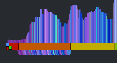
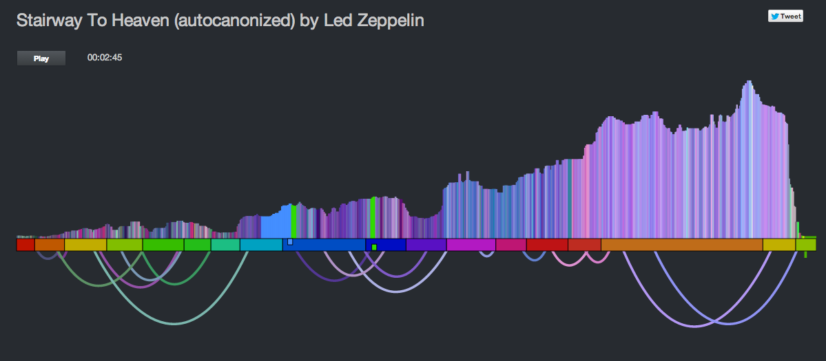
I’ve found with many of these remixing apps, giving the listener a visualization that helps them understand what is happening under the hood is a key part of the hack. The first visualization that accompanied my hack was rather lame:
It showed the beats lined up in a row, colored by the timbral data. The two playback streams were represented by two ‘tape heads’ – the red tape head playing the main stream and the green head showing the canon stream. You could click on beats to play different parts of the song, but it didn’t really give you an idea what was going on under the hood. In the few days since the hackathon, I’ve spent a few hours upgrading the visualization to be something better. I did four things: Reveal more about the song structure, show the song sections, show, the canon graph and animate the transitions.
Reveal more about the song
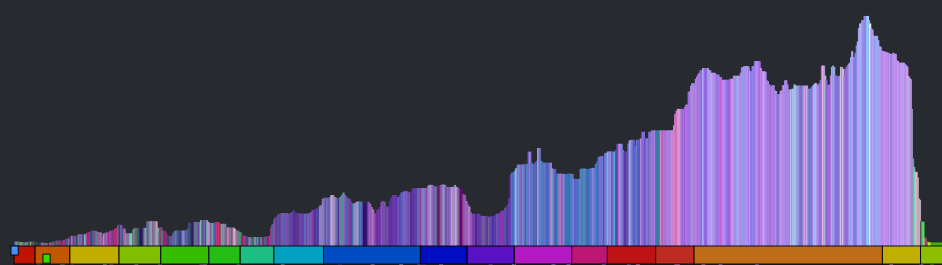
The colored bars don’t really tell you too much about the song. With a good song visualization you should be able to tell the difference between two songs that you know just by looking at the visualization. In addition to the timbral coloring, showing the loudness at each beat should reveal some of the song structure. Here’s a plot that shows the beat-by-beat loudness for the song stairway to heaven.
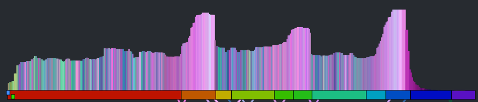
You can see the steady build in volume over the course of the song. But it is still less than an ideal plot. First of all, one would expect the build for a song like Stairway to Heaven to be more dramatic than this slight incline shows. This is because the loudness scale is a logarithmic scale. We can get back some of the dynamic range by converting to a linear scale like so:
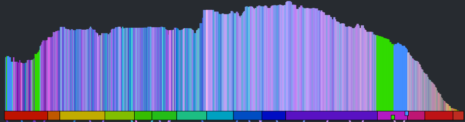
This is much better, but the noise still dominates the plot. We can smooth out the noise by taking a windowed average of the loudness for each beat. Unfortunately, that also softens the sharp edges so that short events, like ‘the drop’ could get lost. We want to be able to preserve the edges for significant edges while still eliminating much of the noise. A good way to do this is to use a median filter instead of a mean filter. When we apply such a filter we get a plot that looks like this:
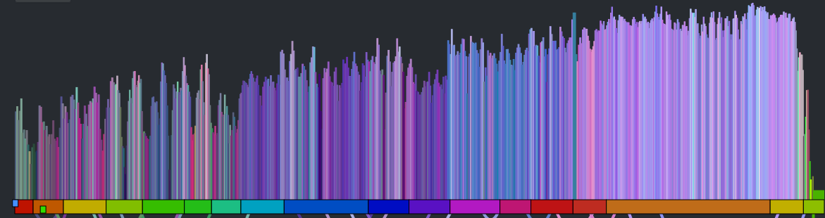
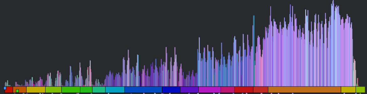
The noise is gone, but we still have all the nice sharp edges. Now there’s enough info to help us distinguish between two well known songs. See if you can tell which of the following songs is ‘A day in the life’ by The Beatles and which one is ‘Hey Jude’ by The Beatles.
Which song is it? Hey Jude or A day in the Life?
Which song is it? Hey Jude or A day in the Life?
Show the song sections
As part of the visualization upgrades I wanted to show the song sections to help show where the canon phrase boundaries are. To do this I created a the simple set of colored blocks along the baseline. Each one aligns with a section. The colors are assigned randomly.
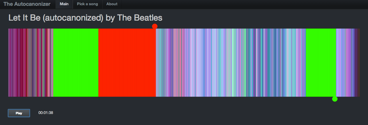
Show the canon graph and animate the transitions.
To help the listener understand how the canon is structured, I show the canon transitions as arcs along the bottom of the graph. When the song is playing, the green cursor, representing the canon stream animates along the graph giving the listener a dynamic view of what is going on. The animations were fun to do. They weren’t built into Raphael, instead I got to do them manually. I’m pretty pleased with how they came out.
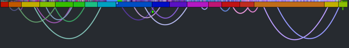
All in all I think the visualization is pretty neat now compared to where it was after the hack. It is colorful and eye catching. It tells you quite a bit about the structure and make up of a song (including detailed loudness, timbral and section info). It shows how the song will be represented as a canon, and when the song is playing it animates to show you exactly what parts of the song are being played against each other. You can interact with the vizualization by clicking on it to listen to any particular part of the canon.
Wrapping up – this was a fun hack and the results are pretty unique. I don’t know of any other auto-canonizing apps out there. It was pretty fun to demo that hack at the SXSW Music Hack Championships too. People really seemed to like it and even applauded spontaneously in the middle of my demo. The updates I’ve made since then – such as fixing the audio glitches and giving the visualization a face lift make it ready for the world to come and visit. Now I just need to wait for them to come.
Anti-preferences in regional listening
Posted by Paul in data, The Echo Nest, zero ui on February 28, 2014
In previous posts, we’ve seen that different regions of the country can have different listening preferences. So far we’ve looked at the distinctive artists in any particular region. Perhaps equally interesting is to look at artists that get much fewer listens in a particular region than you would expect. These are the regional anti-preferences, the artists that are generally popular across the United States, but get much less love in a particular part of the country.
To find these artists, we merely look for artists that drop the furthest in rank on the top-most-played chart for a region when compared to the whole U.S. For example, we can look at the top 50 artists in the United States, and find those artists of the 50 that drop furthest in rank on the New Hampshire chart. Try it yourself. Here are the results:
Artists listened to more in United States than they are in New Hampshire
| # | Artist | Rank in United States |
Rank in New Hampshire |
Delta |
|---|---|---|---|---|
| 1 | R. Kelly | 42 | 720 | -678 |
| 2 | 2Pac | 45 | 243 | -198 |
| 3 | Usher | 46 | 205 | -159 |
| 4 | Coldplay | 36 | 155 | -119 |
| 5 | Chris Brown | 37 | 120 | -83 |
R. Kelly is ranked the 42nd most popular artist in the U.S., but in New Hampshire he’s the 720th most popular, a drop of 678 positions on the chart making him the most ignored artist in New Hampshire.
We can do this for each of the states in the United States and of course we can put them on a map. Here’s a map that shows the most ignored artist of the U.S. top-50 artist in each state.
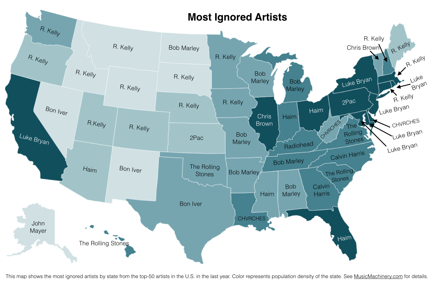
What can we do with this information? If we know where a music listener lives, but we know nothing else about them, we can potentially improve their listening experience by giving them music based upon their local charts instead of the global or national charts. We can also improve the listening even if we don’t know where the listener is from. As we can see from the map, certain artists are polarizing artists, liked in some circles and disliked in others. If we eliminate the polarizing artists for a listener that we know nothing about, we can reduce the risk of musically offending the listener. Of course, once we know a little bit about the music taste of a listener we can greatly improve their recommendations beyond what we can do based solely on demographic info such as the listener location.
Future work There are a few more experiments that I’d like to try with regard to exploring regional preferences. In particular I think it’d be fun to generate an artist similarity metric based solely on regional listening behaviors. In this world, Juicy J, the southern rapper, and Hillsong United, the worship band would be very similar since they both get lots of listens from people in Memphis. A few readers have suggested alternate scoring algorithms to try, and of course it would be interesting to repeat these experiments for other parts of the world. So much music data, so little time! However, this may be the last map I make for a while since the Internet must be getting sick of ‘artists on a map’ by now.
Credit and thanks to Randal Cooper (@fancycwabs) for creating the first set of anti-preference maps. Check out his blog and the Business Insider article about his work.
The data for the map is drawn from an aggregation of data across a wide range of music services powered by The Echo Nest and is based on the listening behavior of a quarter million online music listeners.
Favorite Artists vs Distinctive Artists by State
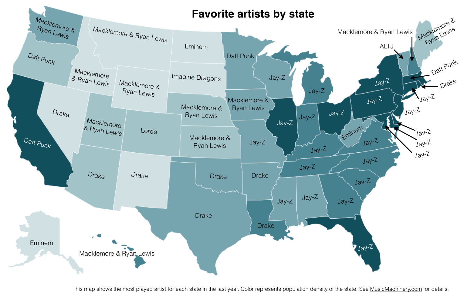
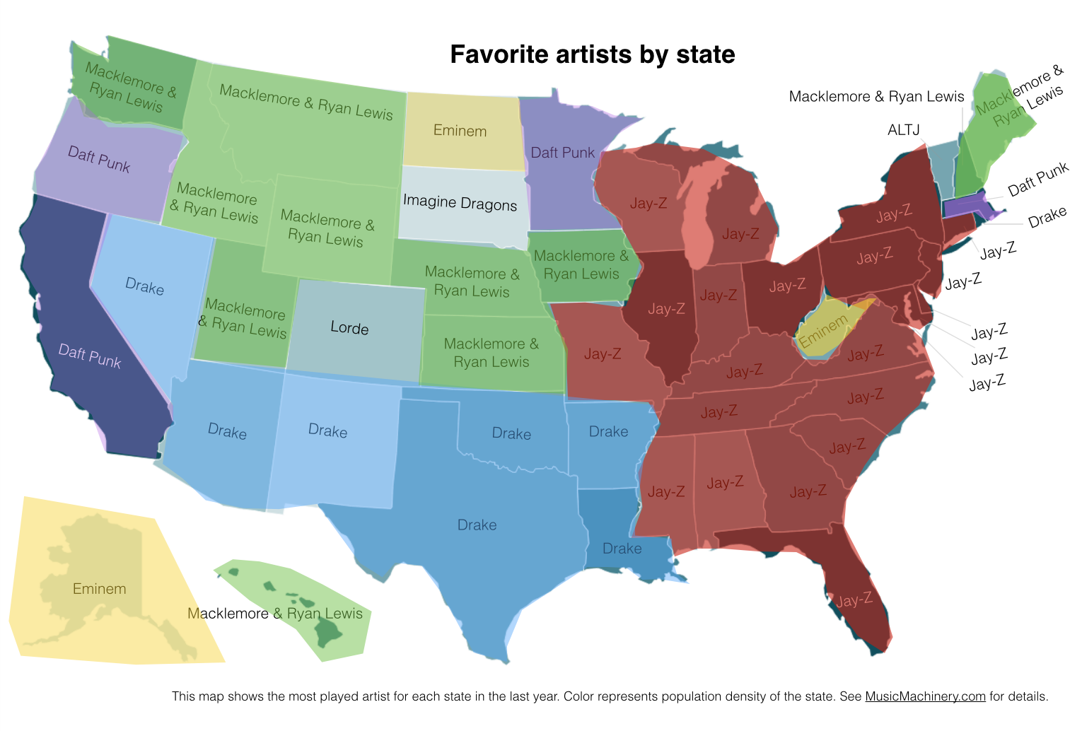
In my recent regional listening preferences post I published a map that showed the distinctive artists by state. The map was rather popular, but unfortunately was a source of confusion for some who thought that the map was showing the favorite artist by state. A few folks have asked what the map of favorite artists per state would look like and how it would compare to the distinctive map. Here are the two maps for comparison.
Favorite Artists by State
This map shows the most played artist in each state over the last year. It is interesting to see the regional differences in favorite artists and how just a handful of artists dominates the listening of wide areas of the country.
Most Distinctive Artists by State
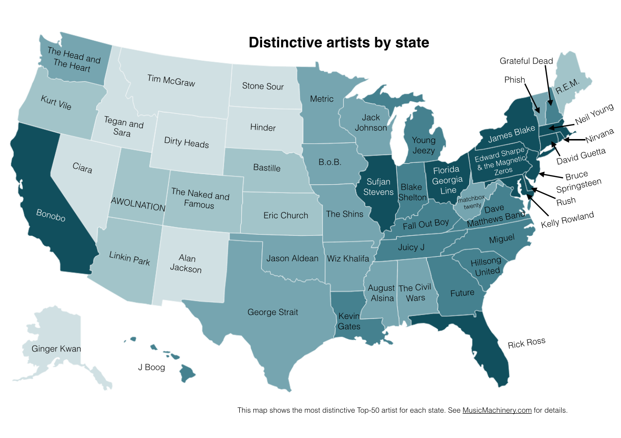
This is the previously published map that shows the artists that are listened to proportionally more frequently in a particular state than they are in all of the United States.
The data for both maps is drawn from an aggregation of data across a wide range of music services powered by The Echo Nest and is based on the listening behavior of a quarter million online music listeners.
It is interesting to see that even when we consider just the most popular artists, we can see regionalisms in listening preferences. I’ve highlighted the regions with color on this version of the map:
Favorite Artist Regions
Exploring age-specific preferences in listening
Earlier this week we looked at how gender can affect music listening preferences. In this post, we continue the tour through demographic data and explore how the age of the listener tells us something about their music taste.
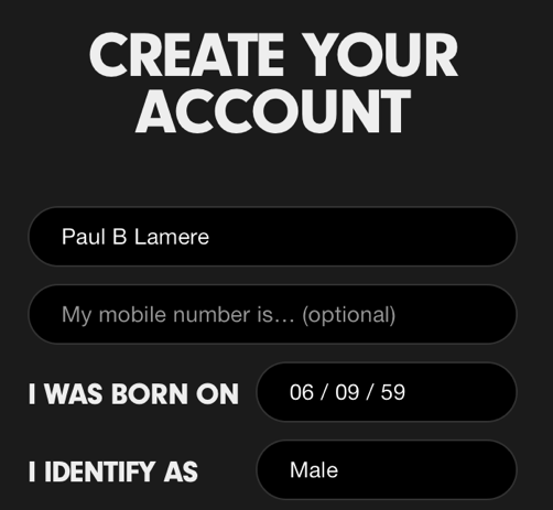
Where does the age data come from? As part of the enrollment process for most music services, the user is asked for a few pieces of demographic data, including gender and year-of-birth. As an example, here’s a typical user-enrollment screen from a popular music subscription service:
Is this age data any good? The first thing we need to do before we get too far with analyzing the age data is to get a feel for how accurate it is. If new users are entering random values for their date of birth then we won’t be able to use the listener’s age for anything useful. For this study, I looked at the age data submitted by several million listeners. This histogram shows the relative number of users by year of birth.
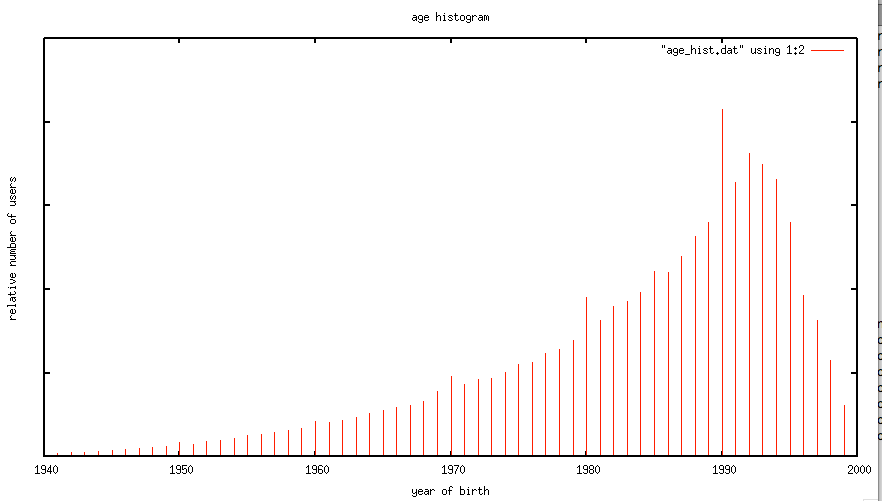
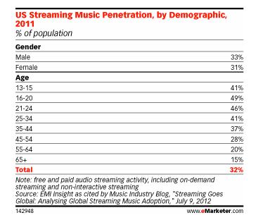
The first thing I notice is the curve has the shape one would expect. The number of listeners in each age bucket increases as the listener gets younger until around age 21 or so, at which points it drops off rapidly. The shape of the curve aligns with the data from this study by EMI in 2011 that shows the penetration of music streaming service by age demographic. This is a good indicator that our age data is an accurate representation of reality.
However, there are a few anomalies in the age data. There are unexpected peaks at each decade – likely due to people rounding their birth year to the nearest decade. A very small percentage (0.01 %) indicate that they are over 120 years old, which is quite unlikely. Despite this noise, the age data looks to be a valid and fairly accurate representation, in the aggregate, of the age of listeners. We should be able to use this data to understand how age impacts listening.
Does a 64-year-old listen to different music than a 13-year-old?
One would expect that people of different ages would have different music tastes. Let’s see if we can confirm this with our data. For starters, lets compare the average listening habits of 64-year-old listeners to that of the aggregate listening habits of the 13-year-old listener. For this experiment I selected 5,000 listeners in each age category, and aggregated their normalized artist plays to find the most-frequently-played artists. As expected, you can see that 64-year-old listeners have different tastes than 13-year-old listeners.
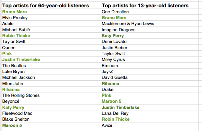
The top artists for the average 64-year-old listener include a mix of currently popular artists along with a number of artists from years gone by. While the top artists for the average 13-year-old includes only the most current artists. Still, there are seven artists (shown in bold) that overlap in the top 20 – an overlap rate of about 35%. This 35% overlap is consistent across all ranges of top artists for the two groups. No matter if we look at the top 100 or the top 1000 artists – there’s about a 35% overlap between the listening of 13- and 64-year-olds.

I suspect that 35% overlap is actually an overstatement of the real overlap between 13- and 64-year-olds. There are a few potential confounding effects:
- There’s a built-in popularity bias in music services. If you go to any popular music service you will see that they all feature a number of playlists filled with popular music. Playlists like The Billboard Top 100, The Viral 50, The Top Tracks, Popular New Releases etc. populate the home page or starting screen for most music services. This popularity bias inflates the apparent interest in popular music so, for instance, it may look like a 64-year-old is more interested in popular music than they really are because they are curious about what’s on all of those featured playlists.
- The age data isn’t perfect – for instance, there are certainly a number of people that we think are 64-years-old but are not. This will skew the results to artists that are more generally popular. We don’t really know how big this affect is, but it is certainly non-zero.
- People share listening accounts – this is perhaps the biggest confounding factor – that 64-year-old listener may be listening to music with their kids, their grand-kids, their neighbors and friends which means that not all of those plays should count as plays by a 64-year-old. Again, we don’t know how big this effect is, but it is certainly non-zero.
Let’s pause and have a listen to some music. First the favorite music of a typical 64-year-old listener:
And now the favorite music of a typical 13-year-old listener:
Finding the most distinctive artists
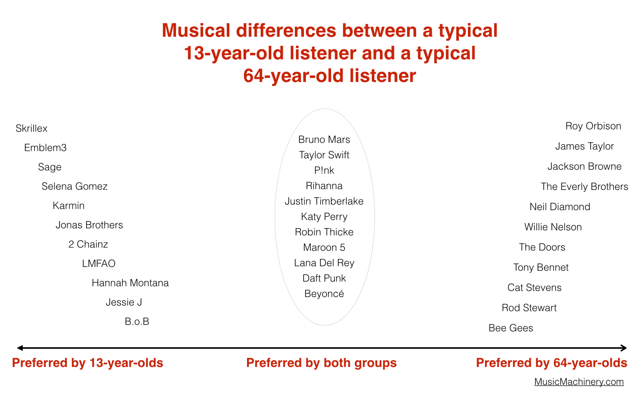
Perhaps more interesting than looking at how the two ages overlap in listening, is to look at how they differ – what are the artists that a 64-year-old will listen to that are rarely, if ever, listened to by a 13-year-old and vice versa. These are the most distinctive artists.
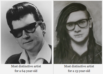
We can find the distinctive artists by identifying the artists in the top 100 of one group that fall the furthest in ranking in the other group. For example Skrillex is the 40th most listened to artist for the typical 13-year-old listener, but for 64-year-old listeners, Skrillex falls all the way to the 3,937 most listened to artist, making Skrillex one of the most distinguishing artist between the two groups of listeners. Likewise, Roy Orbison is the 42nd most listened to artist among 64-year-olds. He drops to position 4,673 among 13-year-olds making him one of the distinguishing artists that separate the 64-year-old from the 13-year-old.
We can use this technique to create playlists of artists that separate the 13-year-old from the 64-year-olds. Are you a 13-year-old, having a party and really wish that grandma would go to another room? Try this playlist:
Are you a 64-year-old and you want all of those 13 year-olds at the party to go home? Try this playlist:
We can also use this data to bring these two groups together. We can find the music that is liked the most among the two groups. We can do this by ordering artists by their worst ranking among the two groups. Artists like Skrillex and Roy Orbison fall to the bottom of the list since each is poorly ranked by one of the groups, while artists like Katy Perry and Bruno Mars rise to the top because they are favored by both groups.
Again, the confounding factors mentioned previously will bias the shared lists to more popular music. Nevertheless, if you are trying to make a playlist of music that will please both a 64-year-old and a 13-year-old, and you know nothing else about their music taste, this is probably your best bet.
Artists that are favored by both 64-year-old and 13-year-old listeners are: Bruno Mars, Taylor Swift, P!nk, Rihanna, Justin Timberlake, Katy Perry, Robin Thicke, Maroon 5, Lana Del Rey, Daft Punk, Beyoncé, Drake, Luke Bryan, Adele, Macklemore & Ryan Lewis, Miley Cyrus, David Guetta, Lorde, Jay-Z, Usher
We can sum up the differences between the two groups in this graphic:
Broadening our view
We’ve shown that, as expected, 13-year-olds and 64-year-olds have different listening preferences. We can apply the same techniques across the range of age demographics typically used by marketers. We can find the most distinctive artists for each demographic bucket. It is interesting to see the progression of music taste over time. For instance, it is clear that something happens to a music listener between the 25 to 34 and 35 to 44 age buckets. The typical listener goes from hipster (Lumineers, Vampire Weekend, The National), to old (Pearl Jam, U2, Bon Jovi).
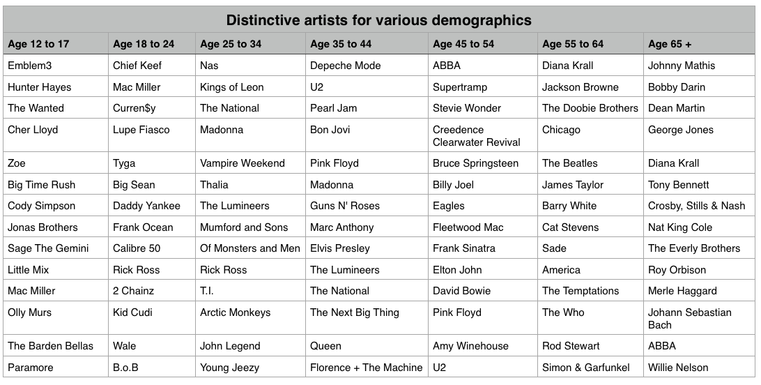
It is interesting to look at the starting year for artists in each of these buckets to get a sense of how the artist’s own age relates to the age of their fans:
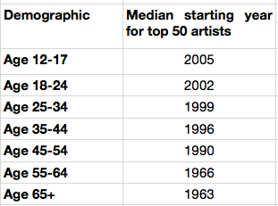
My take-way from this is that no matter how old you are, you don’t like the music from the 70s and the 80s so much.
Most homogenous Artists
We can also find the artists that are most acceptable across all demographics. These are the artists that are liked by more listeners in all of the groups. Like in the 13/64-year-old example, we can find these artists by ordering them by their worst ranking among all the demographic groups.
Most homogeneous artists: Bruno Mars, Rihanna, Katy Perry, Lana Del Rey, Beyoncé, P!nk, Jay-Z, Macklemore & Ryan Lewis, Daft Punk, Maroon 5, Justin Timberlake, Robin Thicke, David Guetta, Luke Bryan, Taylor Swift, Drake, Adele, Imagine Dragons, Miley Cyrus, Lorde
This is essentially the list of the most popular artists but with the most polarizing artists from any one demographic removed. If you don’t know the age of your listener, and you want to give the listener a low risk listening experience, these artists are a good place to start. And yes … this results in a somewhat bland, non-adventurous listening session – that’s the point. But as soon as you know a bit about the true listening preference of a new listener, you can pivot away from the bland and give them something much more in line with their music taste.
Rounding out the stats
There are a few more interesting bits of data we an pull out related to the age of the listener
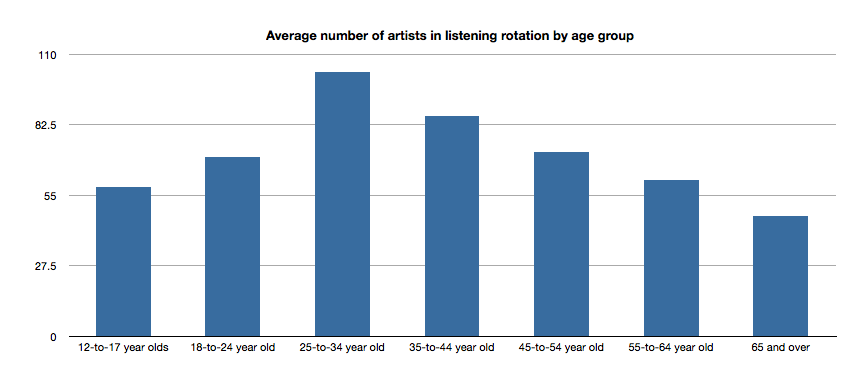
Average number of artists in listening rotation
The typical 25- to 34-year old listener has more artists in active rotation than any other age group, while the 65+ listeners have the least.
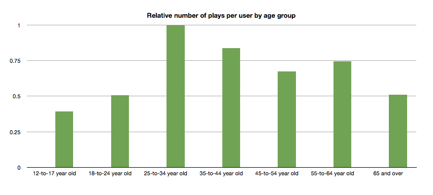
Relative number of plays per user by age group
Likewise, the typical 25- to 34-year-old listener plays more music than any other category.
Tying it all up …
This quick tour through the ages confirms our thinking that the age of a listener plays a significant role in the type of music that they listen to. We can use this information to find music that is distinctive for a particular demographic. We can also use this information to help find artists that may be acceptable to a wide range of listeners. But we should be careful to consider how popularity bias may affect our view of the world. And perhaps most important of all, people don’t like music from the 70s or 80s so much.
Gender Specific Listening
Posted by Paul in data, Music, music information retrieval, recommendation, research, The Echo Nest, zero ui on February 10, 2014
One of the challenges faced by a music streaming service is to figure out what music to play for the brand-new listener. The first listening experience of a new listener can be critical to gaining that listener as a long time subscriber. However, figuring out what to play for that new listener is very difficult because often there’s absolutely no data available about what kind of music that listener likes. Some music services will interview the new listener to get an idea of their music tastes.
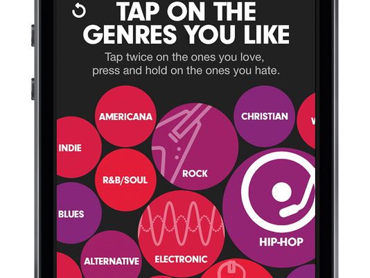
Selecting your favorite genres is part of the nifty user interview for Beat’s music
However, we’ve seen that for many listeners, especially the casual and indifferent listeners, this type of enrollment may be too complicated. Some listeners don’t know or care about the differences between Blues, R&B and Americana and thus won’t be able to tell you which they prefer. A listener whose only experience in starting a listening session is to turn on the radio may not be ready for a multi-screen interview about their music taste.
So what can a music service play for a listener when they have absolutely no data about that listener? A good place to start is to play music by the most popular artists. Given no other data, playing what’s popular is better than nothing. But perhaps we can do better than that. The key is in looking at the little bit of data that a new listener will give you.
For most music services, there’s a short user enrollment process that gets some basic info from the listener including their email address and some basic demographic information. Here’s the enrollment box for Spotify:
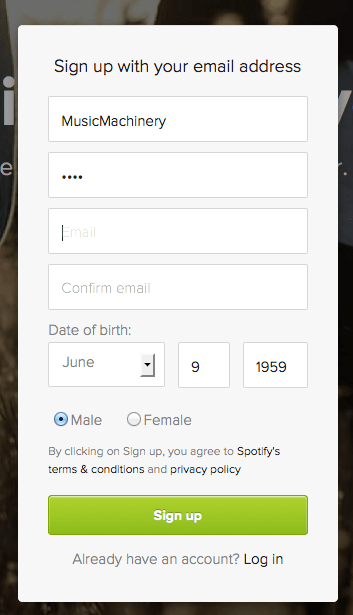
Included in this information is the date of birth and the gender of the listener. Perhaps we can use basic demographic data to generate a slightly more refined set of artists. For starters, lets consider gender. Let’s try to answer the question: If we know that a listener is male or female does that increase our understanding of what kind of music they might like? Let’s take a look.
Exploring Gender Differences in Listening
Do men listen to different music than women do? Anecdotally, we can think of lots of examples that point to yes – it seems like more of One Direction’s fans are female, while more heavy metal fans are male, but lets take a look at some data to see if this is really the case.
The Data – For this study, I looked at the recent listening of about 200 thousand randomly selected listeners that have self-identified as either male or female. From this set of listeners, I tallied up the number of male and female listeners for each artist and then simply ranked the artists in order or listeners. Here’s a quick look at the top 5 artists by gender.
Top 5 artists by gender
| Rank | All | Male | Female |
|---|---|---|---|
| 1 | Rihanna | Eminem | Rihanna |
| 2 | Bruno Mars | Daft Punk | Bruno Mars |
| 3 | Eminem | Jay-Z | Beyoncé |
| 4 | Katy Perry | Bruno Mars | Katy Perry |
| 5 | Justin Timberlake | Drake | P!nk |
Among the top 5 we see that the Male and Female listeners only share one artist in common:Bruno Mars. This trend continues as we look at the top 40 artists. Comparing lists by eye can be a bit difficult, so I created a slopegraph visualization to make it easier to compare. Click on this image to see the whole slopegraph:

click for full chart
Looking at the top 40 charts artists we see that more than a quarter of the artists are gender specific. Artists that top the female listener chart but are missing on the male listener chart include: Justin Bieber, Demi Lovato, Shakira, Britney Spears, One Direction, Christina Aguilera, Ke$ha, Ciara, Jennifer Lopez, Avril Lavigne and Nicki Minaj. Conversely, artists that top the male listener chart but are missing on the top 40 female listener chart include: Bob Marley, Kendrick Lamar, Wiz Khalifa, Avicii, T.I. Queen, J.Cole, Linkin Park, Kid Cudi and 50 Cent. While some artists seem to more easily cross gender lines like Rihanna, Justin Timberlake, Lana Del Rey and Robin Thicke.
No matter what size chart we look at – whether it is the top 40, top 200 or the top 1000 artists – about 30% of artists on a gender-specific chart don’t appear on the corresponding chart for the opposite gender. Similarly, about 15% of the artists that appear on a general chart of top artists will be of low relevance to a typical listener based on these gender-listening differences.
What does this all mean? If you don’t know anything about a listener except for their gender, you can reduce the listener WTFs by 15% for a typical listener by restricting plays to artists from the gender specific charts. But perhaps even more importantly, we can use this data to improve the listening experience for a listener even if we don’t know a listener’s gender at all. Looking at the data we see that there are a number of gender-polarizing artists on any chart. These are artists that are extremely popular for one gender, but not popular at all for the other. Chances are that if you play one of these polarizing artists for a listener that you know absolutely nothing about, 50% of the time you will get it wrong. Play One Direction and 50% of the time the listener won’t like it, just because 50% of the time the listener is male. This means that we can improve the listening experience for a listener, even if we don’t know their gender by eliminating the gender skewing artists and replacing them with more gender neutral artists.
Let’s see how this would affect our charts. Here are the new Top 40 artists when we account for gender differences.
| Rank | Old Rank | Artist |
|---|---|---|
| 1 | 2 | Bruno Mars |
| 2 | 1 | Rihanna |
| 3 | 5 | Justin Timberlake |
| 4 | 4 | Katy Perry |
| 5 | 6 | Drake |
| 6 | 15 | Chris Brown |
| 7 | 3 | Eminem |
| 8 | 8 | P!nk |
| 9 | 11 | David Guetta |
| 10 | 14 | Usher |
| 11 | 17 | Maroon 5 |
| 12 | 7 | Jay-Z |
| 13 | 13 | Adele |
| 14 | 9 | Beyoncé |
| 15 | 12 | Lil Wayne |
| 16 | 23 | Lana Del Rey |
| 17 | 25 | Robin Thicke |
| 18 | 24 | Pitbull |
| 19 | 27 | The Black Eyed Peas |
| 20 | 19 | Lady Gaga |
| 21 | 20 | Michael Jackson |
| 22 | 10 | Daft Punk |
| 23 | 18 | Miley Cyrus |
| 24 | 22 | Macklemore & Ryan Lewis |
| 25 | 28 | Coldplay |
| 26 | 16 | Taylor Swift |
| 27 | 26 | Calvin Harris |
| 28 | 21 | Alicia Keys |
| 29 | 29 | Imagine Dragons |
| 30 | 30 | Britney Spears |
| 31 | 44 | Ellie Goulding |
| 32 | 31 | Kanye West |
| 33 | 42 | J. Cole |
| 34 | 41 | T.I. |
| 35 | 52 | LMFAO |
| 36 | 32 | Shakira |
| 37 | 35 | Bob Marley |
| 38 | 54 | will.i.am |
| 39 | 36 | Ke$ha |
| 40 | 39 | Wiz Khalifa |
Artists promoted to the chart due to replace gender-skewed artists are in bold. Artists that were dropped from the top 40 are:
- Avicii – skews male
- Justin Bieber – skews female
- Christina Aguilera – skews female
- One Direction – skews female
- Demi Lovato – skews female
Who are the most gender skewed artists?
The Top 40 is a fairly narrow slice of music. It is much more interesting to look at how listening can skew across a much broader range of music. Here I look at the top 1,000 artists listened to by males and the top 1,000 artists listened to by females and find the artists that have the largest change in rank as they move from the male chart to the female chart. Artists that lose the most rank are artists that skew male the most, while artists that gain the most rank skew female.
Top male-skewed artists:
artists that skew towards male fans
- Iron Maiden
- Rage Against the Machine
- Van Halen
- N.W.A
- Jimi Hendrix
- Limp Bizkit
- Wu-Tang Clan
- Xzibit
- The Who
- Moby
- Alice in Chains
- Soundgarden
- Black Sabbath
- Stone Temple Pilots
- Mobb Deep
- Queens of the Stone Age
- Ice Cube
- Kavinsky
- Audioslave
- Pantera
Top female-skewed artists:
artists that skew towards female fans
- Danity Kane
- Cody Simpson
- Hannah Montana
- Emily Osment
- Playa LImbo
- Vanessa Hudgens
- Sandoval
- Miranda Lambert
- Sugarland
- Aly & AJ
- Christina Milian
- Noel Schajris
- Maria José
- Jesse McCartney
- Bridgit Mendler
- Ashanti
- Luis Fonsi
- La Oreja de Van Gogh
- Michelle Williams
- Lindsay Lohan
Gender-skewed Genres
By looking at the genres of the most gender skewed artists we can also get a sense of which genres are most gender skewed as well. Looking at the genres of the top 1000 artists listened to by male listeners and the top 1000 artists with female listeners we identify the most skewed genres:
Genres most skewed to female listeners:
- Pop
- Dance Pop
- Contemporary Hit Radio
- Urban Contemporary
- R&B
- Hot Adult Contemporary
- Latin Pop
- Teen Pop
- Neo soul
- Latin
- Pop rock
- Contemporary country
Genres most skewed to male listeners:
- Rock
- Hip Hop
- House
- Album Rock
- Rap
- Pop Rap
- Indie Rock
- Funk Rock
- Gangster Rap
- Electro house
- Classic rock
- Nu metal
Summary
This study confirms what we expected – that there are differences in gender listening. For mainstream listening about 30% of the artists in a typical male’s listening rotation won’t be found in a typical female listening rotation and vice versa. If we happen to know a listener’s gender and nothing else, we can improve their listening experience somewhat by replacing artists that skew to the opposite gender with more neutral artists. We can even improve the listening experience for a listener that we know absolutely nothing about – not even their gender – by replacing gender-polarized artists with artists that are more accepted by both genders.
Of course when we talk about gender differences in listening, we are talking about probabilities and statistics averaged over a large number of people. Yes, the typical One Direction fan is female, but that doesn’t mean that all One Direction fans are female. We can use gender to help us improve the listening experience for a brand new user, even if we don’t know the gender of that new user. But I suspect the benefits of using gender for music scheduling is limited to helping with the cold start problem. After a new user has listened to a dozen or so songs, we’ll have a much richer picture of the type of music they listen to – and we may discover that the new male listener really does like to listen to One Direction and Justin Bieber and that new female listener is a big classic rock fan that especially likes Jimi Hendrix.
update – 2/13 – commenter AW suggested that the word ‘bias’ was too loaded a term. I agree and have changed the post replacing ‘bias’ with ‘difference’
Creative hacking
My hack at the MIDEM Music Hack Day this year is what I’d call a Creative Hack. I built it, not because it answered any business use case or because it demonstrated some advanced capability of some platform or music tech ecosystem, I built it because I was feeling creative and I wanted to express my creativity in the best way that I can which is to write a computer program. The result is something I’m particularly proud of. It’s a dynamic visualization of the song Burn by Ellie Goulding. Here’s a short, low-res excerpt, but I strongly suggest that you go and watch the full version here: Cannes Burn
[youtube http://www.youtube.com/watch?v=Fys0RGi3kA8&feature=youtu.be]Unlike all of the other hacks that I’ve built, this one feels really personal to me. I wasn’t just trying to solve a technical problem. I was trying to capture the essence of the song in code, trying to tell its story and maybe even touch the viewer. The challenge wasn’t in the coding it was in the feeling.
After every hack day, I’m usually feeling a little depressed. I call it post-hacking depression. It is partially caused by being sleep deprived for 48 hours, but the biggest component is that I’ve put my all into something for 48 hours and then it is just over. The demo is done, the code is checked into github, the app is deployed online and people are visiting it (or not). The thing that just totally and completely took over my life for two days is completely gone. It is easy to reflect back on the weekend and wonder if all that time and energy was worth it.
Monday night after the MIDEM hack day was over I was in the midst of my post-hack depression sitting in a little pub called Le Crillon when a guy came up to me and said “I saw your hack. It made me feel something. Your hack moved me.”
Cannes Burn won’t be my post popular hack, nor is it my most challenging hack, but it may be my favorite hack because I was able to write some code and make somebody that I didn’t know feel something.
Attention Deficit Radio
Posted by Paul in code, data, events, fun, hacking, music hack day, The Echo Nest on December 8, 2013
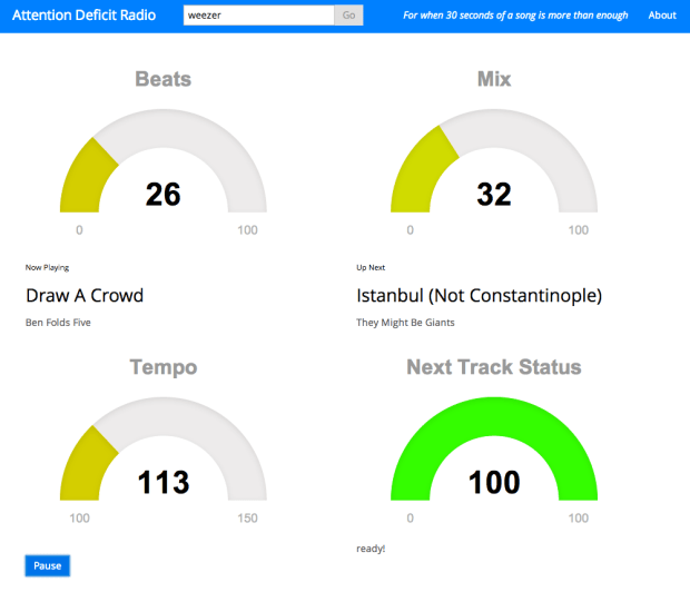
This weekend, I’ve been in London, attending the London Music Hack Day. For this weekend’s hack, I was inspired by daughter’s music listening behavior – when she listens to music, she is good for the first verse or two and the chorus, but after that, she’s on to the next song. She probably has never heard a bridge. So for my daughter, and folks like her with short attention spans, I’ve built Attention Deficit Radio. ADR creates a Pandora-like radio station based upon a seed artist, but doesn’t bother you by playing whole songs. Instead, after about 30 seconds or so, it is on to the next song. The nifty bit is that ADR will try to beat-match and crossfade between the songs giving you a (hopefully) seamless listening experience as you fly through the playlist. Of course those with short attention spans need something to look at while listening, so ADR has lots of gauges that show the radio status – it shows the current beat, the status of the cross-fade, tempo and song loading status.
There may be a few rough edges, and the paint is not yet dry, but give Attention Deficit Radio a try if you have a short listening attention span.
