How to avoid demo fail
So you’ve spent all weekend working on an awesome hack. It is demo time. You have exactly 2 mins to show it off to your hacking peers. You are at the podium, you look out at the faces in the crowd that are anticipating your demo. And nothing works. The 2 minutes stretch to two hours as you wait for that web page with your hack to load. You stammer a “what you would see if this was working” explanation and you leave the stage to a smattering of applause a much more humble person.

As one of the organizers for the Music Hack Day hackathon, I’ve sat through about 500 music hack demos in the last few years and I’ve probably seen at least 50 demo failures. Most of them could have been avoided with just a little bit of preparation. So here’s a list of the most common ways for demos to fail and how you can avoid them.
Hardware Failures
Hooking your computer up to a projector and audio projector should be easy, but sometimes it can be the most vexing of all. If you have the opportunity, do an A/V check before the demo session so you will have all the kinks worked out. Here are the most common failures:
- Missing Adapter – Don’t be surprised if you get to the podium to give your demo and the only thing there is a VGA connector. It never hurts to have an adapter that works with your computer/device in your pocket just in case. (but if you leave your adapter at the podium, you will never see it again).

- Projector won’t sync – it is the worst feeling in the world to connect your laptop to a projector and have it not see the projector. You should know how to force your computer to detect displays.
- No Internet – you are sitting in the audience hitting refresh on your demo web page ever 3 seconds. All is well. It is your turn to give your demo, you close your laptop, walk up to the podium, open it up, plug it in and find that your web page is no longer loading. I’ve see this happen dozens of times. It is easy to forget that when you close your laptop you may lose your network connection and may have to re-login to the local Internet provider before you get access. If you are running a non-web based demo that needs the Internet, this may be hard to notice. What’s worse, when there’s a big demo audience, with lots of laptops, iPads and iPhones, you may no longer even be able to reconnect to the local network. All the local IPs may be used up.

- Non-mirrored display – Lots of hackers have dual display setups. This can work against you when it is time to give a demo. What you see on your laptop in front of you is not what your audience can see. Moreover, the display topology probably won’t match the demo room layout so you may find you can’t even find a way to get your mouse onto the proper screen. Before you give a demo, make sure display mirroring is on. Pro-tip – on a Mac hit CMD-F1 to toggle mirror mode.
- Unexpected display resolution – Projectors usually have a much lower resolution than your desktop. If you are running your demo in a browser, usually you can adjust to a lower resolution, but if your app is written to expect a fixed display size (such as common with a 3D library, or Processing), your app may just not work. Be especially careful if your app needs to switch into fullscreen mode.
- Colors don’t show properly – I’ve seen demos with beautiful visualizations fail because projectors couldn’t show the colors well. If you are relying on colors and textures in your app an A/V check is mandatory.

- No audio jack – At a Music Hack Day you can expect that there will be an audio jack that pipes your laptop audio to the P/A system, but this is not always the case for other hacking events. If you are at a non-music hacking event, double check to make sure that there is an adequate audio hookup. There’s nothing that sounds worse than a demo where you have to hold a microphone up to your laptop speakers so the audience can hear your music.
- Audio Problems – (Added on 12/6/11) (This tip from Yuli Levtov). For those doing hacks based on certain audio-based programming languages e.g. Pure Data, SuperCollider, MaxMSP etc., plugging and un-plugging the mini-jack in a laptop can make these applications behave strangely, as some OSs think the soundcard is being swapped.The solution to this is either a) use a USB soundcard and plug into the headphone jack output at the podium, or b) leave a headphone splitter (small, inexpensive piece of kit) plugged into the headphone output of your laptop at all times, and simply plug the podium minijack into the headphone splitter when you come to give your demo. This will prevent your OS thinking the soundcard has changed, and avoid any nasty needs to re-boot your whole music masterpiece.
- Too many things to hook up – No, you probably don’t need your power supply for a 2 minute demo. Probably don’t need your mouse either. Think twice about that turntable, those lasers, the full rack of keyboards and midi sequencers. Every extra item you bring to the podium doubles the chances of demo fail. Some of the best hacks ever were essentially slide show presentations

Podium Failures
Even if you have successfully hooked up your gear to the projector and audio you are not out of the woods yet. Giving a demo at a podium can be tricky
- Can’t type and hold a microphone at the same time – it is hard enough to type in front of a room full of people. The adrenalin is flowing and your hands are shaking. It is ten times worse if you are also trying to hold a microphone while typing. If there’s a podium or clip on microphone use it. Don’t try to type with a handheld microphone.

- That’s no podium, that’s a table – sometimes there’s no podium, your laptop will be on a desk. You can chose to give your demo standing up and do crouch typing, or sit at the desk where no one will be able to see you. Be ready for unusual setups.

- Notificatus Interruptus – Don’t forget to turn off growl, email and twitter clients that like to put up friendly messages in the middle of your demo.

- No place to put my mouse – If you really need to use a mouse, be ready to find that there’s no room at the podium for a mouse and a laptop.

- It’s chaos up there! – When timing is tight, you’ll find that you are trying to setup your demo while the previous demo is tearing down and while the MC is at the same time trying to get the on deck demo ready. Too many people, too many things to setup, too little time make for a very stressful couple of minutes. Don’t get flustered.

Presentation Failures
Once you have everything setup and connected properly it is time to give actually give your demo. There are still ways to snatch success from the jaws of failure:
- Practice – Giving a demo can be challenging. You are standing at a podium in front of a couple hundred people. Your showing off something that you’ve only just finished building. There may be bugs that you need to work around, the screen may be at the wrong resolution, your hands may be shaking. You may get flustered because the audio volume was too low. With all of this stuff going on, you will forget to demo that cool feature, or you will run out of time before you get to the showstopper. The key to a great demo is Practice Practice Practice. Know what you are going to demo, know what the results will be. Know what you are going to say. Time it, give yourself a few extra seconds of time. Run through it all 10 times.

- Tell us what your demo does – You’ve been living your demo all weekend, you know what it does, but the 200 people in the audience don’t. Tell us what it does. Tell us in a couple of different ways. Make it clear why it is new, cool and worth paying attention to.

- Budget the time properly – You have 2 minutes. We don’t need to know about the github issue you had. We don’t need to know about the difficulties you had installing numpy and scipy. Get to the meat of the demo.
- Don’t waste time telling us about what you failed to do – I’ve heard lots of demos where I was told about this nifty feature that they couldn’t get to work. Don’t demo your failures, demo you successes.
- Make your demo do one thing – Two minutes is not a long time. Especially when you are showing something complex. You may have 5 nifty features in your demo, but you will never be able to demo them all. Pick the coolest feature in your demo and plan to show it a couple of times in a couple of different ways.

- Demo it! – Don’t tell us what your demo is going to do. Show it to us.

- Be enthusiastic – Excitement is contagious. If you are excited about what you are showing, we will get excited too. If you are bored, we will be checking our twitter feed.

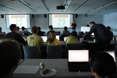
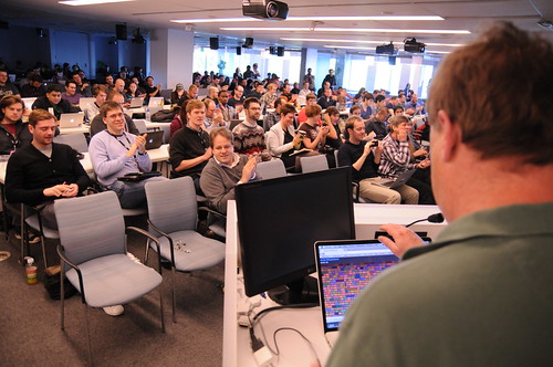
Music Hack Day Boston 2011
Music Hack Day Boston 2011 is in the can. But what a weekend it was. 250 hackers from all over New England and the world gathered at the Microsoft NERD in Cambridge MA for a weekend of hacking on music. Over the course of the weekend, fueled by coffee, red bull, pizza and beer, we created 56 extremely creative music hacks that we demoed in a 3 hour music demo extravaganza at the end of the day on Sunday.

Music Hack Day Boston is held at the Microsoft NERD in Cambridge MA. This is a perfect hacking space – with a large presentation room for talks and demos, along with lots of smaller rooms and nooks and crannies for hackers to camp out .

Hackers started showing up at 9AM on Saturday morning and by 10AM hundreds of hackers were gathered and ready to get started.

After some intelligent and insightful opening remarks by the MC, about 20 companies and organizations gave 5 minute lightening workshops about their technology.
There were a few new (to Music Hack Day) companies giving workshops: Discogs announced Version 2 of their API at the Music Hack Day; Shoudio – the location based audio platform. Peachnote – and API for accessing symbolic music ngram data; EMI who were making a large set of music and data available for hackers as part of their OpenEMI initiative; the Free Music Archive showed their API to give access to 40,000 creative commons licensed songs and WinAmp – showed their developer APIs and network.

After lunch, hacking began in earnest. Some organizations held in-depth workshops giving a deeper dive in to their technologies. Hacking continued in to the evening after shifting to the over night hacking space at The Echo Nest.

Hackers were ensconced in their nests while one floor below there was a rager DJ’d by Ali Shaheed Muhammad (one third of A Tribe called Quest).

Thanks to the gods of time, we were granted one extra hour over night to use to hack or to sleep. Nevertheless, there were many bleary eyes on Sunday morning as hackers arrived back at the NERD to finish their hacks.

Finally at 2:30 PM at 25+ hours of hacking, we were ready to show our hacks.There was an incredibly diverse set of hacks including new musical instruments, new social web sites, new ways to explore for music. The hacks spanned from the serious to the whimsical. Here are some of my favorites.

Free Music Archive Radio – this hack uses the Echo Nest and the Creative Commons licensed music of the Free Music Archive to create interesting playlists for use anywhere.
Mustachiness – Can you turn music into a mustache? The answer is yes. This hack uses sophisticated moustache caching technology to create the largest catalog of musical mustaches in history.

Bohemian Rhapsichord – Turning a popular song into a musical instrument. This is my hack. It lets you play Bohemian Rhapsody like you’ve never played it before.
Spartify – Host a Party and let people choose what songs to play on Spotify. No more huddling in front of one computer or messing up the queue!

Snuggle – I want you to snuggle this. Synchronize animated GIFs to jams of the future. These guys get the prize for most entertaining patter during their demo.

Drinkify – Never listen to music alone again – This app has gone viral. Han, Lindsay and Matt built an app to scratch their own itch. Drinkify automatically generates the perfect cocktail recipe to accompany any music.

Peachnote Musescore and Noteflight search – searching by melody in the two social music score communities.
bitbin – Create and share short 8-bit tunes
The Videolizer – music visualizer that syncs dancing videos to any song. Tristan’s awesome hack – he built a video time stretcher allowing you to synchronize any video that has a soundtrack to a song. The demos are fantastic.
The Echo Nest Prize Winners
Two hacks received the Echo Nest prizes:
unity-echonest – An echonest + freemusicarchive dynamic soundtrack plugin for Unity3D projects. This was a magical demo. David Nunez created a Unity3D plugin that dynamically generates in game soundtracks using the Echo Nest playlist API and music from the Free Music Archive. Wow!

MidiSyncer – sync midi to echo nest songs. Art Kerns built An iPhone app that lets you choose a song from your iTunes library, retrieves detailed beat analysis information from Echo Nest for the song, and then translates that beat info to MIDI clock as the song plays. This lets you sync up an electronic music instrument such as a drum machine or groovebox to a song that’s playing on your iPhone. So wow! Play a song on your iPod and have a drum machine play in sync with it. Fantastic!

Hardware Hacks
Some really awesome hardware hacks.
Neurofeedback – Electroencephalogram + strobe goggles + Twilio Chat Bot + Max/MSP patches which control Shephard-risset rhythms and binaural beats
Sonic Ninja – Zebra Tube Awesomeness – John Shirley develops PVC helmholtz resonator while hacking a WiiMote and bluetooth audio transmission.

SpeckleSounds – Super-sensitive 3D Sound Control w/ Lasers! Yes, with lasers.
Kinect BeatWheel – Control a quantized looping sample with your arm

Demo Fail
There were a few awesome hacks that were cursed by the demo demi gods. Great ideas, great hacks, frustrating (for the hacker) demos. Here are some of the best demo fail hacks .
Kinetic – Kinetic Typography driven by user selected music and text. This was a really cool hack that was plagued by a podium display issue leading to a demi-demo-fail. But the Olin team regrouped and posted a video of the app.
BetterTaste – improve your Spotify image – this was an awesome idea – use a man-in-the-middle proxy to intercept those embarassing scrobbles. Unfortunately Arkadiy had a network disconnect that lead to a demo fail.
Tracker – Connect your turntable to the digital world. Automatically identifies tracks, saves mp3s, and scrobbles plays, while displaying a beautiful UI that’s visible from across the room, or across the web. Perhaps the most elaborate of the demos – with a real Hi Fi setup including a turntable. But something wasn’t clicking, so Abe had to tell us about it instead of showing it.

Carousel – tell the story behind your pictures – it was a display fail – but luckily Johannes had a colleague who had his back and re-gave the demo. That’s what hacker friends are for.

This was a fantastic weekend. Thanks to Thomas Bonte of MuseScore for taking these super images. Special thanks to the awesome Echo Nest crew lead by Elissa for putting together this event, staffing it and making it run like clockwork. It couldn’t have happened without her. I was particularly proud of The Echo Nest this week. We created some awesome hacks, threw a killer party, and showed how to build the future of music while having a great time. What a place to work!
Bohemian Rhapsichord – a Music Hack Day Hack
Posted by Paul in code, events, Music, The Echo Nest on November 6, 2011
It is Music Hack Day Boston this weekend. I worked with my daughter Jennie (of Jennie’s Ultimate Roadtrip fame) to build a music hack. This year we wanted to build a hack that actually made music. And so we built Bohemian Rhapsichord.

Bohemian Rhapsichord is a web app that turns the song Bohemian Rhapsody into a musical instrument. It uses TheEcho Nest analyzer to break the song into segments of quasi-stable musical events. It then shows these as an array of colored tiles (where the colors are based on timbre) that you can interact with like a musical instrument.

If you click on a tile, you play that portion of the song (or hold down shift or control and play tiles just by mousing over them). You can bind different segments to keys letting you play the ‘instrument’ with your keyboard too (See the FAQ for all the details). You can re-sort the tiles based on a few criteria (sequential order, by loudness, duration or by similarity to the last played note). It is a fun way to make music based on one of the best songs in the world.
The app makes use of the very new (and not always the most stable) web audio API. Currently, the only browser that I know that supports the web audio API is Chrome. The app is online so give it a try: Bohemian Rhapsichord
Speechiness – is it banjo or banter?
Posted by Paul in Music, The Echo Nest on November 4, 2011
There’s no bigger buzz kill when listening to a playlist of songs by your favorite artists than to find that you are no longer listening to music, but instead to some radio interview the drummer of the band gave to some local radio station in 1963. If you’ve listened to much Internet radio this has probably happened to you. An algorithmic playlisting engine may know that it is time to play a track by The Beatles, but it probably doesn’t know which tracks in the Beatles discography are music and which ones are interviews, and so sooner or later you’ll find yourself listening to Ringo talking about his new haircut instead of listening to While My Guitar Gently Weeps.

To help deal with this type of problem, The Echo Nest has just pushed out a new analysis attribute called Speechiness. Speechiness is a number between zero and one that indicates how likely a particular audio file is speech. Whenever you analyze a track with the Echo Nest analyzer, the track will be assigned a speechiness score. If the track has a high speechiness score, it is probably mostly speech, if it has a low score it is mostly non-speech. This speechiness parameter is a pretty good way to distinguish between music tracks and non-music tracks. As an example, lets look at tracks by comedian and banjo player Steve Martin. Steve has a large collection of comedy tracks, but he’s also an accomplished blue grass banjo player (What’s the difference between a chain saw and a banjo? You can turn a chain saw off.). We took 35 Steve Martin tracks and calculated the speechiness of them all and ordered them by increasing speechiness. Here’s a plot of the speechiness for these tracks:

You can see there’s a nice stable flat zone of low speechiness tracks – these are the banjo and blue grass ones and a stable flat zone of high speechiness tracks – the standup comedy. In between are some hybrid tracks – like Ramblin man – a comedy routine with a banjo accompaniment. I created a web page where you can audition the tracks to see how well the speechiness attribute has separated the banjo from the banter.

I think it is quite cool how the speechiness attribute was able to separate the music from the spoken word.
Trying this yourself
Brian put together a quick demo that lets you calculate the speechiness of any track that’s on SoundCloud. Brian put the demo together in an hour so he says it is ‘totally buggy and hacky’ – but so far it has worked great for me. Just enter the URL to any SoundCloud tracks, wait a half-a-minute and see the speechiness score. A result in the green is probably music (or some other non-speech audio), while a result in the red is speech.
 The demo is pretty cool. Go to speechiness.echonest.com to try it out. If you don’t have any SoundCloud tracks handy, here are some tracks to try (expect these direct links to take 30 seconds to load since the speechiness web app is triggering a full song analysis on page load):
- hiddenvalley/obama
- kfw/variations-for-oud-synthesizer-1-excerpt
- bwhitman/16-holy-night/
- hardwell/tiesto-bt-love-comes-again-hardwell
{
    "response": {
        "status": {
            "code": 0,
            "message": "Success",
            "version": "4.2"
        },
        "track": {
            "analyzer_version": "3.08d",
            "artist": "The Beatles",
            "artist_id": "AR6XZ861187FB4CECD",
            "audio_summary": {
                "analysis_url": "https://echonest-analysis.s3.amazonaws.com/TR/TRAVQYP13369CD8BDC/3/full.json?Signature=EEiMYDzPquMmlW7fJlLvdWKI6PI%3D&Expires=1320409614&AWSAccessKeyId=AKIAJRDFEY23UEVW42BQ",
                "danceability": 0.37855052706867015,
                "duration": 54.999549999999999,
                "energy": 0.85756107654449365,
                "key": 9,
                "loudness": -10.613,
                "mode": 1,
 "speechiness": 0.1824877387165752,
                "tempo": 91.356999999999999,
                "time_signature": 5
            },
            "bitrate": 2425500,
            "id": "TRAVQYP13369CD8BDC",
            "md5": "ec2d40704439f5650b67884e00242d99",
            "release": "Help!",
            "samplerate": 44100,
            "song_id": "SOINKRY12B20E5E547",
            "status": "complete",
            "title": "Dizzy Miss Lizzie"
        }
    }
}
Wrapping up
The speechiness attribute is an alpha release. There may still be some tweaks to the algorithm in the near future. We’ve currently applied the attribute to the top 100,000 or so most popular tracks in The Echo Nest. Once we are totally satisfied with the algorithm we will apply it to all of our many millions of tracks as well as incorporating it into our search and playlisting APIs allowing you to filter and sort results based upon speechiness. In the future you’ll be able to make that Beatles playlist and limit the results to only tracks that have a low speechiness, eliminating the hair cut interviews entirely from your listening rotation (or conversely and perversely you’ll be able to create a playlist with just the hair cut interviews.) Congrats to The Echo Nest Audio team for rolling out this really useful feature.
ISMIR Session – the web
The first session at ISMIR today is on the Web. 4 really interesting sets of papers:
Songle – an active music listening experience
Mastaka Goto presented Songle at ISMIR this morning. Songle is a web site for active music listening and content-based music browsing. Songle takes many of the MIR techniques that researchers have been working on for years and makes it available to non-MIR experts to help them understand music better. You can also use Songle to modify the music. You can interactively change the beat and melody, copy and paste sections. Your edits can be shared with others. Masataka hopes that Songle can serve as a showcase of MIR and music-understanding of technologies and will serve as a platform for other researchers as well. There’s a lot of really powerful music technology behind Songle. I look forward to trying it out. Paper.
Improving Perceptual Tempo estimation with Crowd-Source Annotations
Mark Levy from Last.fm describes the Last.fm experiment to crowd source the gathering of tempo information (fast, slow and BPM) that can be used to help eliminate tempo ambiguity in machine-estimated tempo (typically known as the octave error). They ran their test over 4K songs from a number of genres. So far they’ve had 27K listeners apply 200k labels and bpm estimates. (woah!). Last.fm is releasing this dataset. Very interesting work. Paper
Investigating the similarity space of music artists on the micro-blogosphere
Markus Schedl analyzed 6 million tweets by searching tweets for artist names and conducted a number of experiments to see if artist similarity could be determined based upon these tweets. (They used the Comirva framework to conduct the experiments). Findings: document based techniques work best (cosine similarity, while not always yielding the best result yielded the most stable results). Unsurprisingly adding the term ‘music’ to the twitter search helps a lot (Reducing the CAKE, Spoon and KISS problems). Surprising result is that using tweets for deriving similarity works better than using larger documents derived from web search. Markus suggest that this may be due to the higher information content in the much shorter tweets. Datasets are available. Paper
Music Influence Network Analysis and Rank of Sample-based Music
Nick Bryan from Stanford – trying to understand how songs/artists and genres interact with the sampled-base music (remixes etc). Using data from Whosampled.com – (42K user-generated sample info sets). From this data they created an directed graph and did some network analysis on the graph (centrality / influence) – Hypothesized that there’s a power law distribution of connectivity (typical small-worlds, scale-free distribution with a rich-gets-richer effect). They confirmed this hypothesis. Use Katz Influence to help understand sample-chains. From the song-sample graph, artist sample graphs (who sampled whom) and genre sample graphs (which genres sample from other genres) were derived. With all these graphs, Nick was then able to understand which songs and artists are the most influential (James Brown is king of sampling), surprisingly, the AMEN break is only the second most influential sample. Interesting and fun work. Paper
Music Recommendation and Discovery Remastered – A Tutorial
Posted by Paul in events, Music, recommendation on October 24, 2011
Oscar and I just finished giving our tutorial on music recommendation and discovery at ACM RecSys 2011. Here are the slides:
What is so special about music?
Posted by Paul in Music, recommendation on October 23, 2011
In the Recommender Systems world there is a school of thought that says that it doesn’t matter what type of items you are recommending. For these folks, a recommender is a black box that takes in user behavior data and outputs recommendations. It doesn’t matter what you are recommending – books, music, movies, Disney vacations, or deodorant. According to this school of thought you can take the system that you use for recommending books and easily repurpose it to recommend music. This is wrong. If you try to build a recommender by taking your collaborative filtering book recommender and applying it to music, you will fail. Music is different. Music is special.
Here are 10 reasons why music is special and why your off-the-shelf collaborative filtering system won’t work so well with music.
Huge item space – There is a whole lot of music out there. Industrial sized music collections typically have 10 million songs or more. The iTunes music store boasts 18 million songs. The algorithms that worked so wonderfully on the Netfix Dataset (one of the largest CF datasets released, contain user data for 17,770 movies) will not work so well when having to deal with a dataset that is three orders of magnitude larger.

Very low cost per item – When the cost per item is low, the risk of a bad recommendation is low. If you recommend to me a bad Disney Vacation I am out $10,000 and a week of my time. If you recommend a bad song, I hit the skip button and move on to the next.

Many item types – In the music world, there are many things to recommend: tracks, albums, artists, genres, covers, remixes, concerts, labels, playlists, radio stations other listeners etc.

Low consumption time – A book can take a week to read, a movie may take a few hours to watch, a song may take 3 minutes to listen to. Since I can consume music so quickly, I need lots of recommendations (perhaps 30 an hour) to keep my queue filled, whereas 30 book recommendations may keep me reading for a whole year. This has implications for scaling of a recommender. It also ties in with the low cost per item issue. Because music is so cheap and so quick to consume, the risk of a bad recommendation is very low. A music recommender can afford to be more adventurous than other types of recommenders.

Very high per-item reuse – I’ve read my favorite book perhaps half-a-dozen times, I’ve seen my favorite movie 3 times and I’ve probably listened to my favorite song thousands of times. We listen to music over and over again. We like familiar music. A music recommender has to understand the tension between familiarity and novelty. The Netflix movie recommender will never recommend The Bourne Identity to me because it knows that I already watched it, but a good music playlist recommender had better include a good mix of my old favorites along with new music.

Highly passionate users -There’s no more passionate fan than a music fan. This is a two-edged sword. If your recommender introduce a music fan to new music that they like they will transfer some of their passion to your music service. This is why Pandora has such a vocal and passionate user base. On the other hand, if your recommender adds a Nickelback track to a Led Zeppelin playlist you will have to endure the wrath of the slighted fan.

Highly contextual usage – We listen to music differently in different contexts. I may have an exercising playlist, a working playlist, a driving playlist etc. I may make a playlist to show my friends how cool I am when I have them over for a social gathering. Not too many people go to Amazon looking for a list of books that they can read while jogging. A successful music recommender needs to take context into account.

Consumed in sequences – Listening to songs in order has always been a big part of the music experience. We love playlists, mixtapes, DJ mixes, albums. Some people make their living putting songs into interesting order. Your collaborative filtering algorithm doesn’t have the ability to create coherent, interesting playlists with a mix of new music and old favorites

Large Personal Collections – Music fans often have extremely large personal collections – making it easier for recommendation and discovery tools to understand the detailed music taste of a listener. A personalized movie recommender may start with a list of a dozen rated movies, while a music recommender may be able to recommend music based upon many thousands of plays, ratings skips and bans.

Highly Social – Music is social. People love to share music. They express their identity to others by the music they listen to. They give each other playlists and mixtapes. Music is a big part of who we are.

Music is special – but of course, so are books, movies and Disney vacations – every type of item has its own special characteristics that should be taken into account when building recommendation and discovery tools. There’s no one-size-fits-all recommendation algorithm.
“What do I do with those 10,000,000 songs in my pocket?”
References to Mae West aside, I’m really looking forward to the Industrial Panel being held during the Workshop on Music Recommendation and Discovery. Great set of attendees:
- Amélie Anglade (Soundcloud, GE) moderator
- Eric Bieschke (Pandora, US)
- Douglas Eck (Google Music, US)
- Justin Sinkovich (Epitonic, US)
- Evan Stein (Decibel, UK)
Music Recommendation and Discovery Revisited
Posted by Paul in freakomendation, recommendation on October 22, 2011
I’m off to Chicago to attend the 5th ACM Conference on Recommender Systems. I’m giving a talk with Òscar Celma called Music Recommendation and Discovery Revisited. It is a reprise of the talk we gave 4 years ago at ISMIR 2007 in Austria. Quite a bit has happened in the music discovery space since then so there’s quite a bit of new material. Here’s one of my favorite new slides. 10 points if you can figure out what this slide is all about.
.odp - OpenOffice.org Impress")
It should be a fun talk, and it is always great working with Oscar. We’ll post the slides on Monday.
Search for music by drawing a picture of it

I’ve spent the weekend hacking on a project at Music Hack Day Montreal. For my hack I created an application with the catchy title “Search for music by drawing a picture of it”. The hack lets you draw the loudness profile for a song and the app will search through the Million Song Data Set to find the closest match. You can then listen to the song in Spotify (if the song is in the Spotify collection).
Coding a project in 24 hours is all about compromise. I had some ideas that I wanted to explore to make the matching better (dynamic time warping) and the lookup faster (LSH). But since I actually wanted to finish my hack I’ve saved those improvements for another day. The simple matching approach (Euclidean distance between normalized vectors) works surprisingly well. The linear search through a million loudness vectors takes about 20 seconds, too long for a web app, this can be made palatable with a little Ajax .
The hack day has been great fun, kudos to the Montreal team for putting it all together.
