Archive for category data
My Music Hack Day London hack
Posted by Paul in code, data, events, The Echo Nest on December 4, 2011
It is Music Hack Day London this weekend. However, I am in New England, not Olde England, so I wasn’t able to enjoy in all the pizza, beer and interesting smells that come with a 24 hour long hackathon. But that didn’t keep me from writing code. Since Spotify Apps are the cool new music hacking hotttnesss, I thought I’d create a Spotify related hack called the Artist Picture Show. It is a simple hack – it shows a slide show of artist images while you listen to them. It gets the images from The Echo Nest artist images API and from Flickr. It is a simple app, but I find the experience of being able to see the artist I’m listening too to be quite compelling.

Slightly more info on the hack here.
The Music Matrix – Exploring tags in the Million Song Dataset
Posted by Paul in code, data, Music, The Echo Nest on November 27, 2011
Last month Last.fm contributed a massive set of tag data to the Million Song Data Set. The data set includes:
- 505,216 tracks with at least one tag
- 522,366 unique tags
- 8,598,630 (track – tag) pairs
A popular track like Led Zep’s Stairway to Heaven has dozens of unique tags applied hundreds of times.

There is no end to the number of interesting things you can do with these tags: Track similarity for recommendation and playlisting, faceted browsing of the music space, ground truth for training autotagging systems etc.
I think there’s quite a bit to be learned about music itself by looking at these tags. We live in a post-genre world where most music no longer fits into a nice tidy genre categories. There are hundreds of overlapping subgenres and styles. By looking at how the tags overlap we can get a sense for the structure of the new world of music. I took the set of tags and just looked at how the tags overlapped to get a measure of how often a pair of tags co-occur. Tags that have high co-occurrence represent overlapping genre space. For example, among the 500 thousand tracks the tags that co-occur the most are:
- rap co-occurs with hip hop 100% of the time
- alternative rock co-occurs with rock 76% of the time
- classic rock co-occurs with rock 76% of the time
- hard rock co-occurs with rock 72% of the time
- indie rock co-occurs with indie 71% of the time
- electronica co-occurs with electronic 69% of the time
- indie pop co-occurs with indie 69% of the time
- alternative rock co-occurs with alternative 68% of the time
- heavy metal co-occurs with metal 68% of the time
- alternative co-occurs with rock 67% of the time
- thrash metal co-occurs with metal 67% of the time
- synthpop co-occurs with electronic 66% of the time
- power metal co-occurs with metal 65% of the time
- punk rock co-occurs with punk 64% of the time
- new wave co-occurs with 80s 63% of the time
- emo co-occurs with rock 63% of the time
It is interesting to see how the subgenres like hard rock or synthpop overlaps with the main genre and how all rap overlaps with Hip Hop. Using simple overlap we can also see which tags are the least informative. These are tags that overlap the most with other tags, meaning that they are least descriptive of tags. Some of the least distinctive tags are: Rock, Pop, Alternative, Indie, Electronic and Favorites. So when you tell someone you like ‘rock’ or ‘alternative’ you are not really saying too much about your musical taste.
The Music Matrix
I thought it might be interesting to explore the world of music via overlapping tags, and so I built a little web app called The Music Matrix. The Music Matrix shows the overlapping tags for a tag neighborhood or an artist via a heat map. You can explore the matrix, looking at how tags overlap and listening to songs that fit the tags.

With this app you can enter a genre, style, mood or other type of tag. The app will then find the 24 tags with the highest overlap with the seed and show the confusion matrix. Hotter colors indicate high overlap. Mousing over a cell will show you the percentage overlap between the two corresponding tags and clicking on a cell will play a track that has high tag counts for the two tags. I find that I can learn a lot about a genre of music by looking at the 24 tag neighborhood for a genre and listening to examples. Some interesting neighborhoods to explore are:
You can also explore by moods:
If you are not sure what genre or style is for an artist, you can just start with the top tags for the artist like so:
Use the Music Matrix to explore a new genre of music or to find music that matches a set of styles. Find out how genres overlap. Listen to prototypical examples of different styles. Click on things, have fun. Check it out:
The code for the Music Matrix is on Github. Thanks to Thierry for creating the Million Song Data Set (the best research data set ever created) and thanks to Last.fm for contributing a very nice set of tag data to the data set.
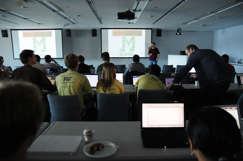
Music Hack Day Boston 2011
Music Hack Day Boston 2011 is in the can. But what a weekend it was. 250 hackers from all over New England and the world gathered at the Microsoft NERD in Cambridge MA for a weekend of hacking on music. Over the course of the weekend, fueled by coffee, red bull, pizza and beer, we created 56 extremely creative music hacks that we demoed in a 3 hour music demo extravaganza at the end of the day on Sunday.

Music Hack Day Boston is held at the Microsoft NERD in Cambridge MA. This is a perfect hacking space – with a large presentation room for talks and demos, along with lots of smaller rooms and nooks and crannies for hackers to camp out .

Hackers started showing up at 9AM on Saturday morning and by 10AM hundreds of hackers were gathered and ready to get started.

After some intelligent and insightful opening remarks by the MC, about 20 companies and organizations gave 5 minute lightening workshops about their technology.
There were a few new (to Music Hack Day) companies giving workshops: Discogs announced Version 2 of their API at the Music Hack Day; Shoudio – the location based audio platform. Peachnote – and API for accessing symbolic music ngram data; EMI who were making a large set of music and data available for hackers as part of their OpenEMI initiative; the Free Music Archive showed their API to give access to 40,000 creative commons licensed songs and WinAmp – showed their developer APIs and network.

After lunch, hacking began in earnest. Some organizations held in-depth workshops giving a deeper dive in to their technologies. Hacking continued in to the evening after shifting to the over night hacking space at The Echo Nest.

Hackers were ensconced in their nests while one floor below there was a rager DJ’d by Ali Shaheed Muhammad (one third of A Tribe called Quest).

Thanks to the gods of time, we were granted one extra hour over night to use to hack or to sleep. Nevertheless, there were many bleary eyes on Sunday morning as hackers arrived back at the NERD to finish their hacks.

Finally at 2:30 PM at 25+ hours of hacking, we were ready to show our hacks.There was an incredibly diverse set of hacks including new musical instruments, new social web sites, new ways to explore for music. The hacks spanned from the serious to the whimsical. Here are some of my favorites.

Free Music Archive Radio – this hack uses the Echo Nest and the Creative Commons licensed music of the Free Music Archive to create interesting playlists for use anywhere.
Mustachiness – Can you turn music into a mustache? The answer is yes. This hack uses sophisticated moustache caching technology to create the largest catalog of musical mustaches in history.

Bohemian Rhapsichord – Turning a popular song into a musical instrument. This is my hack. It lets you play Bohemian Rhapsody like you’ve never played it before.

Spartify – Host a Party and let people choose what songs to play on Spotify. No more huddling in front of one computer or messing up the queue!

Snuggle – I want you to snuggle this. Synchronize animated GIFs to jams of the future. These guys get the prize for most entertaining patter during their demo.

Drinkify – Never listen to music alone again – This app has gone viral. Han, Lindsay and Matt built an app to scratch their own itch. Drinkify automatically generates the perfect cocktail recipe to accompany any music.

Peachnote Musescore and Noteflight search – searching by melody in the two social music score communities.
bitbin – Create and share short 8-bit tunes
The Videolizer – music visualizer that syncs dancing videos to any song. Tristan’s awesome hack – he built a video time stretcher allowing you to synchronize any video that has a soundtrack to a song. The demos are fantastic.
The Echo Nest Prize Winners
Two hacks received the Echo Nest prizes:
unity-echonest – An echonest + freemusicarchive dynamic soundtrack plugin for Unity3D projects. This was a magical demo. David Nunez created a Unity3D plugin that dynamically generates in game soundtracks using the Echo Nest playlist API and music from the Free Music Archive. Wow!

MidiSyncer – sync midi to echo nest songs. Art Kerns built An iPhone app that lets you choose a song from your iTunes library, retrieves detailed beat analysis information from Echo Nest for the song, and then translates that beat info to MIDI clock as the song plays. This lets you sync up an electronic music instrument such as a drum machine or groovebox to a song that’s playing on your iPhone. So wow! Play a song on your iPod and have a drum machine play in sync with it. Fantastic!

Hardware Hacks
Some really awesome hardware hacks.
Neurofeedback – Electroencephalogram + strobe goggles + Twilio Chat Bot + Max/MSP patches which control Shephard-risset rhythms and binaural beats

Sonic Ninja – Zebra Tube Awesomeness – John Shirley develops PVC helmholtz resonator while hacking a WiiMote and bluetooth audio transmission.

SpeckleSounds – Super-sensitive 3D Sound Control w/ Lasers! Yes, with lasers.
Kinect BeatWheel – Control a quantized looping sample with your arm

Demo Fail
There were a few awesome hacks that were cursed by the demo demi gods. Great ideas, great hacks, frustrating (for the hacker) demos. Here are some of the best demo fail hacks .
Kinetic – Kinetic Typography driven by user selected music and text. This was a really cool hack that was plagued by a podium display issue leading to a demi-demo-fail. But the Olin team regrouped and posted a video of the app.
BetterTaste – improve your Spotify image – this was an awesome idea – use a man-in-the-middle proxy to intercept those embarassing scrobbles. Unfortunately Arkadiy had a network disconnect that lead to a demo fail.
Tracker – Connect your turntable to the digital world. Automatically identifies tracks, saves mp3s, and scrobbles plays, while displaying a beautiful UI that’s visible from across the room, or across the web. Perhaps the most elaborate of the demos – with a real Hi Fi setup including a turntable. But something wasn’t clicking, so Abe had to tell us about it instead of showing it.

Carousel – tell the story behind your pictures – it was a display fail – but luckily Johannes had a colleague who had his back and re-gave the demo. That’s what hacker friends are for.

This was a fantastic weekend. Thanks to Thomas Bonte of MuseScore for taking these super images. Special thanks to the awesome Echo Nest crew lead by Elissa for putting together this event, staffing it and making it run like clockwork. It couldn’t have happened without her. I was particularly proud of The Echo Nest this week. We created some awesome hacks, threw a killer party, and showed how to build the future of music while having a great time. What a place to work!
Search for music by drawing a picture of it

I’ve spent the weekend hacking on a project at Music Hack Day Montreal. For my hack I created an application with the catchy title “Search for music by drawing a picture of it”. The hack lets you draw the loudness profile for a song and the app will search through the Million Song Data Set to find the closest match. You can then listen to the song in Spotify (if the song is in the Spotify collection).
Coding a project in 24 hours is all about compromise. I had some ideas that I wanted to explore to make the matching better (dynamic time warping) and the lookup faster (LSH). But since I actually wanted to finish my hack I’ve saved those improvements for another day. The simple matching approach (Euclidean distance between normalized vectors) works surprisingly well. The linear search through a million loudness vectors takes about 20 seconds, too long for a web app, this can be made palatable with a little Ajax .
The hack day has been great fun, kudos to the Montreal team for putting it all together.
Looking for the Slow Build
This is the second in a series of posts exploring the Million Song Dataset.

Every few months you’ll see a query like this on Reddit – someone is looking for songs that slowly build in intensity. It’s an interesting music query since it is primarily focused on what the music sounds like. Since we’ve analyzed the audio of millions and millions of tracks here at The Echo Nest we should be able to automate this type of query. One would expect that Slow Build songs will have a steady increase in volume over the course of a song, so lets look at the loudness data for a few Slow Build songs to confirm this intuition. First, here’s the canonical slow builder: Stairway to Heaven:
 The green line is the raw loudness data, the blue line is a smoothed version of the data. Clearly we see a rise in the volume over the course of the song. Let’s look at another classic Slow Build – The Hall Of the Mountain King – again our intuition is confirmed:

Looking at a non-Slow Build song like Katy Perry’s California Gurls we see that the loudness curve is quite flat by comparison:

Of course there are other aspects beyond loudness that a musician may use to build a song to a climax – tempo, timbre and harmony are all useful, but to keep things simple I’m going to focus only on loudness.
Looking at these plots it is easy to see which songs have a Slow Build. To algorithmically identify songs that have a slow build, we can use a technique similar to the one I described in The Stairway Detector. It is a simple algorithm that compares the average loudness of the first half of the song to the average loudness of the second half of the song. Songs with the biggest increase in average loudness rank the highest. For example, take a look at a loudness plot for Stairway to Heaven. You can see that there is a distinct rise in scores from the first half to the second half of the song (the horizontal dashed lines show the average loudness for the first and second half of the song). Calculating the ramp factor we see that Stairway to Heaven scores an 11.36 meaning that there is an increase in average loudness of 11.36 decibels between the first and the second half of the song.
This algorithm has some flaws – for instance it will give very high scores to ‘hidden track’ songs. Artists will sometimes ‘hide’ a track at the end of a CD by padding the beginning of the track with a few minutes of silence. For example, this track by ‘Fudge Tunnel’ has about five minutes of silence before the band comes in.

Clearly this song isn’t a Slow Build, our simple algorithm is fooled. To fix this we need to introduce a measure of how straight the ramp is. One way to measure the straightness of a line is to calculate the Pearson correlation for the loudness data as a function of time. XY Data with correlation that approaches one (or negative one) is by definition, linear. This nifty wikipedia visualization of the correlation of different datasets shows the correlation for various datasets:
 We can combine the correlation with our ramp factors to generate an overall score that takes into account the ramp of the song as well as the straightness of the ramp. The overall score serves as our Slow Build detector. Songs with a high score are Slow Build songs. I suspect that there are better algorithms for this so if you are a math-oriented reader who is cringing at my naivete please set me and my algorithm straight.
Armed with our Slow Build Detector, I built a little web app that lets you explore for Slow Build songs. The app – Looking For The Slow Build – looks like this:

The application lets you type in the name of your favorite song and will give you a plot of the loudness over the course of the song, and calculates the overall Slow Build score along with the ramp and correlation. If you find a song with an exceptionally high Slow Build score it will be added to the gallery. I challenge you to get at least one song in the gallery.
You may find that some songs that you think should get a high Slow Build score don’t score as high as you would expect. For instance, take the song Hoppipolla by Sigur Ros. It seems to have a good build, but it scores low:

It has an early build but after a minute it has reached it’s zenith. The ending is symmetrical with the beginning with a minute of fade. This explains the low score.
Another song that builds but has a low score is Weezer’s The Angel and the One.

This song has a 4 minute power ballad build – but fails to qualify a a slow build because the last 2 minutes of the song are nearly silent.
Finding Slow Build songs in the Million Song Dataset
Now that we have an algorithm that finds Slow Build songs, lets apply it to the Million Song Dataset. I can create a simple MapReduce job in Python that will go through all of the million tracks and calculate the Slow Build score for each of them to help us find the songs with the biggest Slow Build. I’m using the same framework that I described in the post “How to Process a Million Songs in 20 minutes“. I use the S3 hosted version of the Million Song Dataset and process it via Amazon’s Elastic MapReduce using mrjob – a Python MapReduce library. Here’s the mapper that does almost all of the work, the full code is on github in cramp.py:
    def mapper(self, _, line):
        """ The mapper loads a track and yields its ramp factor """
        t = track.load_track(line)
        if t and t['duration'] > 60 and len(t['segments']) > 20:
            segments = t['segments']
            half_track = t['duration'] / 2
            first_half = 0
            second_half = 0
            first_count = 0
            second_count = 0

            xdata = []
            ydata = []
            for i in xrange(len(segments)):
                seg = segments[i]
                seg_loudness = seg['loudness_max'] * seg['duration']

                if seg['start'] + seg['duration'] <= half_track:
                    seg_loudness = seg['loudness_max'] * seg['duration']
                    first_half += seg_loudness
                    first_count += 1
                elif seg['start'] < half_track and seg['start'] + seg['duration'] > half_track:
                    # this is the nasty segment that spans the song midpoint.
                    # apportion the loudness appropriately
                    first_seg_loudness = seg['loudness_max'] * (half_track - seg['start'])
                    first_half += first_seg_loudness
                    first_count += 1

                    second_seg_loudness = seg['loudness_max'] * (seg['duration'] - (half_track - seg['start']))
                    second_half += second_seg_loudness
                    second_count += 1
                else:
                    seg_loudness = seg['loudness_max'] * seg['duration']
                    second_half += seg_loudness
                    second_count += 1

                xdata.append( seg['start'] )
                ydata.append( seg['loudness_max'] )

            correlation = pearsonr(xdata, ydata)
            ramp_factor = second_half / half_track - first_half / half_track
            if YIELD_ALL or ramp_factor > 10 and correlation > .5:
                yield (t['artist_name'], t['title'], t['track_id'], correlation), ramp_factor
This code takes less than a half hour to run on 50 small EC2 instances and finds a bucketload of Slow Build songs. I’ve created a page of plots of the top 500 or so Slow Build songs found by this job. There are all sorts of hidden gems in there. Go check it out:
Looking for the Slow Build in the Million Song Dataset
The page has 500 plots all linked to Spotify so you can listen to any song that strikes your fancy. Here are some my favorite discoveries:
Respighi’s The Pines of the Appian Way
I remember playing this in the orchestra back in high school. It really is sublime. Click the plot to listen in Spotify.

Maria Friedman’s Play The Song Again
So very theatrical

Mandy Patinkin’s Rock-A-Bye Your Baby With A Dixie Melody
Another song that seems to be right off of Broadway – it has an awesome slow build.


- The Million Song Dataset – deep data about a million songs
- The Stairway Index – my first look at this stuff about 2 years ago
- How to process a million songs in 20 minutes – a blog post about how to process the MSD with mrjob and Elastic Map Reduce
- Looking for the Slow Build – a simple web app that calculates the Slow Build score and loudness plot for just about any song
- cramp.py – the MapReduce code for calculating Slow Build scores for the MSD
- Looking for the Slow Build in the Million Song Dataset – 500 loudness plots of the top Slow Builders
- Top Slow Build songs in the Million Song Dataset – the top 6K songs with a Slow Build score of 10 and above
- A Spotify collaborative playlist with a bunch of Slow Build songs in it. Feel free to add more.
How to process a million songs in 20 minutes
The recently released Million Song Dataset (MSD), a collaborative project between The Echo Nest and Columbia’s LabROSA is a fantastic resource for music researchers. It contains detailed acoustic and contextual data for a million songs. However, getting started with the dataset can be a bit daunting. First of all, the dataset is huge (around 300 gb) which is more than most people want to download. Second, it is such a big dataset that processing it in a traditional fashion, one track at a time, is going to take a long time. Even if you can process a track in 100 milliseconds, it is still going to take over a day to process all of the tracks in the dataset. Luckily there are some techniques such as Map/Reduce that make processing big data scalable over multiple CPUs. In this post I shall describe how we can use Amazon’s Elastic Map Reduce to easily process the million song dataset.
The Problem

From 'Creating Music by Listening' by Tristan Jehan
For this first experiment in processing the million song data set I want to do something fairly simple and yet still interesting. One easy calculation is to determine each song’s density – where the density is defined as the average number of notes or atomic sounds (called segments) per second in a song. To calculate the density we just divide the number of segments in a song by the song’s duration. The set of segments for a track is already calculated in the MSD. An onset detector is used to identify atomic units of sound such as individual notes, chords, drum sounds, etc. Each segment represents a rich and complex and usually short polyphonic sound. In the above graph the audio signal (in blue) is divided into about 18 segments (marked by the red lines). The resulting segments vary in duration. We should expect that high density songs will have lots of activity (as an Emperor once said “too many notes”), while low density songs won’t have very much going on. For this experiment I’ll calculate the density of all 1 million songs and find the most dense and the least dense songs.
MapReduce
A traditional approach to processing a set of tracks would be to iterate through each track, process the track, and report the result. This approach, although simple, will not scale very well as the number of tracks or the complexity of the per track calculation increases. Luckily, a number of scalable programming models have emerged in the last decade to make tackling this type of problem more tractable. One such approach is MapReduce.
MapReduce is a programming model developed by researchers at Google for processing and generating large data sets. With MapReduce you specify a map function that processes a key/value pair to generate a set of intermediate key/value pairs, and a reduce function that merges all intermediate values associated with the same intermediate key. There are a number of implementations of MapReduce including the popular open sourced Hadoop and Amazon’s Elastic MapReduce.
There’s a nifty MapReduce Python library developed by the folks at Yelp called mrjob. With mrjob you can write a MapReduce task in Python and run it as a standalone app while you test and debug it. When your mrjob is ready, you can then launch it on a Hadoop cluster (if you have one), or run the job on 10s or even 100s of CPUs using Amazon’s Elastic MapReduce. Writing an mrjob MapReduce task couldn’t be easier. Here’s the classic word counter example written with mrjob:
from mrjob.job import MRJob

class MRWordCounter(MRJob):
    def mapper(self, key, line):
        for word in line.split():
            yield word, 1

    def reducer(self, word, occurrences):
        yield word, sum(occurrences)

if __name__ == '__main__':
    MRWordCounter.run()
The input is presented to the mapper function, one line at a time. The mapper breaks the line into a set of words and emits a word count of 1 for each word that it finds. The reducer is called with a list of the emitted counts for each word, it sums up the counts and emits them.
When you run your job in standalone mode, it runs in a single thread, but when you run it on Hadoop or Amazon (which you can do by adding a few command-line switches), the job is spread out over all of the available CPUs.
MapReduce job to calculate density
We can calculate the density of each track with this very simple mrjob – in fact, we don’t even need a reducer step:
class MRDensity(MRJob):
    """ A  map-reduce job that calculates the density """

    def mapper(self, _, line):
        """ The mapper loads a track and yields its density """
        t = track.load_track(line)
        if t:
            if t['tempo'] > 0:
                density = len(t['segments']) / t['duration']
                yield (t['artist_name'], t['title'], t['song_id']), density
(see the full code on github)
The mapper loads a line and parses it into a track dictionary (more on this in a bit), and if we have a good track that has a tempo then we calculate the density by dividing the number of segments by the song’s duration.
Parsing the Million Song Dataset
We want to be able to process the MSD with code running on Amazon’s Elastic MapReduce. Since the easiest way to get data to Elastic MapReduce is via Amazon’s Simple Storage Service (S3), we’ve loaded the entire MSD into a single S3 bucket at http://tbmmsd.s3.amazonaws.com/. (The ‘tbm’ stands for Thierry Bertin-Mahieux, the man behind the MSD). This bucket contains around 300 files each with data on about 3,000 tracks. Each file is formatted with one track per line following the format described in the MSD field list. You can see a small subset of this data for just 20 tracks in this file on github: tiny.dat. I’ve written track.py that will parse this track data and return a dictionary containing all the data.
You are welcome to use this S3 version of the MSD for your Elastic MapReduce experiments. But note that we are making the S3 bucket containing the MSD available as an experiment. If you run your MapReduce jobs in the “US Standard Region” of Amazon, it should cost us little or no money to make this S3 data available. If you want to download the MSD, please don’t download it from the S3 bucket, instead go to one of the other sources of MSD data such as Infochimps. We’ll keep the S3 MSD data live as long as people don’t abuse it.
Running the Density MapReduce job
You can run the density MapReduce job on a local file to make sure that it works:
% python density.py tiny.dat
This creates output like this:
["Planet P Project", "Pink World", "SOIAZJW12AB01853F1"]	3.3800521773317689
["Gleave", "Come With Me", "SOKBZHG12A81C21426"]	7.0173630509232234
["Chokebore", "Popular Modern Themes", "SOGVJUR12A8C13485C"]	2.7012807851495166
["Casual", "I Didn't Mean To", "SOMZWCG12A8C13C480"]	4.4351713380683542
["Minni the Moocher", "Rosi_ das M\u00e4dchen aus dem Chat", "SODFMEL12AC4689D8C"]	3.7249476012698159
["Rated R", "Keepin It Real (Skit)", "SOMJBYD12A6D4F8557"]	4.1905674943168156
["F.L.Y. (Fast Life Yungstaz)", "Bands", "SOYKDDB12AB017EA7A"]	4.2953929132587785
Where each ‘yield’ from the mapper is represented by a single line in the output, showing the track ID info and the calculated density.
Running on Amazon’s Elastic MapReduce
When you are ready to run the job on a million songs, you can run it the on Elastic Map Reduce. First you will need to set up your AWS system. To get setup for Elastic MapReduce follow these steps:
- create an Amazon Web Services account: <http://aws.amazon.com/>
- sign up for Elastic MapReduce: <http://aws.amazon.com/elasticmapreduce/>
- Get your access and secret keys (go to <http://aws.amazon.com/account/> and click on “Security Credentials”)
- Set the environment variables $AWS_ACCESS_KEY_ID and $AWS_SECRET_ACCESS_KEY accordingly for mrjob.
Once you’ve set things up, you can run your job on Amazon using the entire MSD as input by adding a few command switches like so:
% python density.py --num-ec2-instances 100 --python-archive t.tar.gz -r emr 's3://tbmmsd/*.tsv.*' > out.dat
The ‘-r emr’ says to run the job on Elastic Map Reduce, and the ‘–num-ec2-instances 100’ says to run the job on 100 small EC2 instances. A small instance currently costs about ten cents an hour billed in one hour increments, so this job will cost about $10 to run if it finishes in less than an hour, and in fact this job takes about 20 minutes to run. If you run it on only 10 instances it will cost 1 or 2 dollars. Note that the t.tar.gz file simply contains any supporting python code needed to run the job. In this case it contains the file track.py. See the mrjob docs for all the details on running your job on EC2.
The Results
The output of this job is a million calculated densities, one for each track in the MSD. We can sort this data to find the most and least dense tracks in the dataset. Here are some high density examples:
Ichigo Ichie by Ryuji Takeuchi has a density of 9.2 segments/second

Ichigo Ichie by Ryuji Takeuchi
129 by Strojovna 07 has a density of 9.2 segments/second

129 by Strojovna 07
The Feeding Circle by Makaton with a density of 9.1 segments per segment

The Feeding Circle by Makaton
Indeed, these pass the audio test, they are indeed high density tracks. Now lets look at some of the lowest density tracks.
Deviation by Biosphere with a density of .014 segments per second

Deviation by Biosphere
The Wire IV by Alvin Lucier with a density of 0.014 segments per second

The Wire IV by Alvin Lucier
improvisiation_122904b by Richard Chartier with a density of .02 segments per second

improvisation by Richard Chartier
Wrapping up
The ‘density’ MapReduce task is about as simple a task for processing the MSD that you’ll find. Consider this the ‘hello, world’ of the MSD. Over the next few weeks, I’ll be creating some more complex and hopefully interesting tasks that show some of the really interesting knowledge about music that can be gleaned from the MSD.
(Thanks to Thierry Bertin-Mahieux for his work in creating the MSD and setting up the S3 buckets. Thanks to 7Digital for providing the audio samples)
Searching for chilled metal
It seems like every heavy metal band has at least one chill-out song – from Metallica’s Nothing Else Matters to Led Zeppelin’s That’s the Way. These tracks give some relief from the otherwise relentless pounding of the hammer of the gods. It’d be nice to be able to collect up a bunch of these chilled-metal songs into a playlist – perfect for when your mom’s visiting (she tells me that she doesn’t like pounding metal).

ChilLed Zeppelin - Some rights (by-nc-sa) reserved by Heinrich Klaffs
To find chilled metal, we can use The Echo Nest API. The Echo Nest has calculated a wide range of acoustic and musical attributes for millions of songs. One such attribute is energy . We can make a simple song/search query for heavy metal songs that have low energy. These will be our chilled-metal songs that your mom enjoys so much. Here’s the API query:
http://developer.echonest.com/api/v4/song/search?&style=heavy+metal&sort=energy-asc
This query searches for songs by heavy metal artists, and sorts the results in order of ascending energy (so the lowest energy tracks will be returned first). The query does a really good job of finding chilled metal. Here’s a sampling of the results:

Sphinx (The Guardian) by Black Sabbath
[audio http://previews.7digital.com/clips/34/645345.clip.mp3]
Sphinx (The Guardian) by Black Sabbath – energy: 0.0003

Demon Driver reprise by Gillan
[audio http://previews.7digital.com/clips/34/4179195.clip.mp3]
Demon Drive by Gillan – energy: 0.010

The Return by Saxon
[audio http://previews.7digital.com/clips/34/5318312.clip.mp3]
The Return by Saxon – energy: 0.013

Solitude by Judas Priest
[audio http://previews.7digital.com/clips/34/3544312.clip.mp3]
Solitude by Judas Priest – energy: 0.049

Joan of Arc by UFO
[audio http://previews.7digital.com/clips/34/7952114.clip.mp3]
Joan of Arc by UFO – Energy: 0.05

Fear by Black Label Society
[audio http://previews.7digital.com/clips/34/5768332.clip.mp3]
Fear by Black Label Society – Energy – 0.119
You can also use the Echo Nest Playlist API to generate a chilled metal playlist. Here’s a call to create a playlist of chilled metal in XSPF format.
You can toss this playlist into a player like VLC or Songbird that supports XSPF and start listening to chilled metal right away (30 second samples only) like this:
% curl 'http://developer.echonest.com/api/v4/playlist/static?api_key=N6E4NIOVYMTHNDM8J\
   &style=heavy+metal&max_energy=.1\
   &type=artist-description&bucket=id:7digital&bucket=tracks&limit=true\
   &format=xspf' > chilled-metal.xspf
% open chilled-metal.xspf
There you go, you now have all the tools you need to keep your chilled metal queue filled and fresh, almost everything you need to keep your mom happy.
Thanks much to 7Digital for providing audio clips and album art.
Data Mining Music – a SXSW 2012 Panel Proposal
Posted by Paul in data, events, Music, music information retrieval, The Echo Nest on August 15, 2011

I’ve submitted a proposal for a SXSW 2012 panel called Data Mining Music. The PanelPicker page for the talk is here: Data Mining Music. If you feel so inclined feel free to comment and/or vote for the talk. I promise to fill the talk with all sorts of fun info that you can extract from datasets like the Million Song Dataset.
Here’s the abstract:
Data mining is the process of extracting patterns and knowledge from large data sets. It has already helped revolutionized fields as diverse as advertising and medicine. In this talk we dive into mega-scale music data such as the Million Song Dataset (a recently released, freely-available collection of detailed audio features and metadata for a million contemporary popular music tracks) to help us get a better understanding of the music and the artists that perform the music.
We explore how we can use music data mining for tasks such as automatic genre detection, song similarity for music recommendation, and data visualization for music exploration and discovery. We use these techniques to try to answers questions about music such as: Which drummers use click tracks to help set the tempo? or Is music really faster and louder than it used to be? Finally, we look at techniques and challenges in processing these extremely large datasets.
Questions answered:
- What large music datasets are available for data mining?
- What insights about music can we gain from mining acoustic music data?
- What can we learn from mining music listener behavior data?
- Who is a better drummer: Buddy Rich or Neil Peart?
- What are some of the challenges in processing these extremely large datasets?
Flickr photo CC by tristanf
How do you spell ‘Britney Spears’?
Posted by Paul in code, data, Music, music information retrieval, research, The Echo Nest on July 28, 2011
I’ve been under the weather for the last couple of weeks, which has prevented me from doing most things, including blogging. Luckily, I had a blog post sitting in my drafts folder almost ready to go. I spent a bit of time today finishing it up, and so here it is. A look at the fascinating world of spelling correction for artist names.
 In today’s digital music world, you will often look for music by typing an artist name into a search box of your favorite music app. However this becomes a problem if you don’t know how to spell the name of the artist you are looking for. This is probably not much of a problem if you are looking for U2, but it most definitely is a problem if you are looking for Röyksopp, Jamiroquai or Britney Spears. To help solve this problem, we can try to identify common misspellings for artists and use these misspellings to help steer you to the artists that you are looking for.
A spelling corrector in 21 lines of code
A good place for us to start is a post by Peter Norvig (Director of Research at Google) called ‘How to write a spelling corrector‘ which presents a fully operational spelling corrector in 21 lines of Python. (It is a phenomenal bit of code, worth the time studying it). At the core of Peter’s algorithm is the concept of the edit distance which is a way to represent the similarity of two strings by calculating the number of operations (inserts, deletes, replacements and transpositions) needed to transform one string into the other. Peter cites literature that suggests that 80 to 95% of spelling errors are within an edit distance of 1 (meaning that most misspellings are just one insert, delete, replacement or transposition away from the correct word). Not being satisfied with that accuracy, Peter’s algorithm considers all words that are within an edit distance of 2 as candidates for his spelling corrector. For Peter’s small test case (he wrote his system on a plane so he didn’t have lots of data nearby), his corrector covered 98.9% of his test cases.
Spell checking Britney
A few years ago, the smart folks at Google posted a list of Britney Spears spelling corrections that shows nearly 600 variants on Ms. Spears name collected in three months of Google searches. Perusing the list, you’ll find all sorts of interesting variations such as ‘birtheny spears’ , ‘brinsley spears’ and ‘britain spears’. I suspect that some these queries (like ‘Brandi Spears’) may actually not be for the pop artist. One curiosity in the list is that although there are 600 variations on the spelling of ‘Britney’ there is exactly one way that ‘spears’ is spelled. There’s no ‘speers’ or ‘spheres’, or ‘britany’s beers’ on this list.
One thing I did notice about Google’s list of Britneys is that there are many variations that seem to be further away from the correct spelling than an edit distance of two at the core of Peter’s algorithm. This means that if you give these variants to Peter’s spelling corrector, it won’t find the proper spelling. Being an empiricist I tried it and found that of the 593 variants of ‘Britney Spears’, 200 were not within an edit distance of two of the proper spelling and would not be correctable. This is not too surprising. Names are traditionally hard to spell, there are many alternative spellings for the name ‘Britney’ that are real names, and many people searching for music artists for the first time may have only heard the name pronounced and have never seen it in its written form.
Making it better with an artist-oriented spell checker
A 33% miss rate for a popular artist’s name seems a bit high, so I thought I’d see if I could improve on this. I have one big advantage that Peter didn’t. I work for a music data company so I can be pretty confident that all the search queries that I see are going to be related to music. Restricting the possible vocabulary to just artist names makes things a whole lot easier. The algorithm couldn’t be simpler. Collect the names of the top 100K most popular artists. For each artist name query, find the artist name with the smallest edit distance to the query and return that name as the best candidate match. This algorithm will let us find the closest matching artist even if it is has an edit distance of more than 2 as we see in Peter’s algorithm. When I run this against the 593 Britney Spears misspellings, I only get one mismatch – ‘brandi spears’ is closer to the artist ‘burning spear’ than it is to ‘Britney Spears’. Considering the naive implementation, the algorithm is fairly fast (40 ms per query on my 2.5 year old laptop, in python).
Looking at spelling variations
With this artist-oriented spelling checker in hand, I decided to take a look at some real artist queries to see what interesting things I could find buried within. I gathered some artist name search queries from the Echo Nest API logs and looked for some interesting patterns (since I’m doing this at home over the weekend, I only looked at the most recent logs which consists of only about 2 million artist name queries).
Artists with most spelling variations
Not surprisingly, very popular artists are the most frequently misspelled. It seems that just about every permutation has been made in an attempt to spell these artists.
- Michael Jackson – Variations: michael jackson, micheal jackson, michel jackson, mickael jackson, mickal jackson, michael jacson, mihceal jackson, mickeljackson, michel jakson, micheal jaskcon, michal jackson, michael jackson by pbtone, mical jachson, micahle jackson, machael jackson, muickael jackson, mikael jackson, miechle jackson, mickel jackson, mickeal jackson, michkeal jackson, michele jakson, micheal jaskson, micheal jasckson, micheal jakson, micheal jackston, micheal jackson just beat, micheal jackson, michal jakson, michaeljackson, michael joseph jackson, michael jayston, michael jakson, michael jackson mania!, michael jackson and friends, michael jackaon, micael jackson, machel jackson, jichael mackson
- Justin Bieber – Variations: justin bieber, justin beiber, i just got bieber’ed by, justin biber, justin bieber baby, justin beber, justin bebbier, justin beaber, justien beiber, sjustin beiber, justinbieber, justin_bieber, justin. bieber, justin bierber, justin bieber<3 4 ever<3, justin bieber x mstrkrft, justin bieber x, justin bieber and selens gomaz, justin bieber and rascal flats, justin bibar, justin bever, justin beiber baby, justin beeber, justin bebber, justin bebar, justien berbier, justen bever, justebibar, jsustin bieber, jastin bieber, jastin beiber, jasten biber, jasten beber songs, gestin bieber, eiine mainie justin bieber, baby justin bieber,
- Red Hot Chili Peppers – Variations: red hot chilli peppers, the red hot chili peppers, red hot chilli pipers, red hot chilli pepers, red hot chili, red hot chilly peppers, red hot chili pepers, hot red chili pepers, red hot chilli peppears, redhotchillipeppers, redhotchilipeppers, redhotchilipepers, redhot chili peppers, redhot chili pepers, red not chili peppers, red hot chily papers, red hot chilli peppers greatest hits, red hot chilli pepper, red hot chilli peepers, red hot chilli pappers, red hot chili pepper, red hot chile peppers
- Mumford and Sons – Variations: mumford and sons, mumford and sons cave, mumford and son, munford and sons, mummford and sons, mumford son, momford and sons, modfod and sons, munfordandsons, munford and son, mumfrund and sons, mumfors and sons, mumford sons, mumford ans sons, mumford and sonns, mumford and songs, mumford and sona, mumford and, mumford &sons, mumfird and sons, mumfadeleord and sons
- Katy Perry – Even an artist with a seemingly very simple name like Katy Perry has numerous variations: katy perry, katie perry, kate perry, kathy perry, katy perry ft.kanye west, katty perry, katy perry i kissed a girl, peacock katy perry, katyperry, katey parey, kety perry, kety peliy, katy pwrry, katy perry-firework, katy perry x, katy perry, katy perris, katy parry, kati perry, kathy pery, katey perry, katey perey, katey peliy, kata perry, kaity perry
Some other most frequently misspelled artists:
- Britney Spears
- Linkin Park
- Arctic Monkeys
- Katy Perry
- Guns N’ Roses
- Nicki Minaj
- Muse
- Weezer
- U2
- Oasis
- Moby
- Flyleaf
- Seether
- byran adams – ryan adams
- Underworld – Uverworld
Visualizing the active years of popular artists
Posted by Paul in data, Music, The Echo Nest, visualization on June 21, 2011
This week the Echo Nest is extending the data returned for an artist to include the active years for an artist. For thousands of artists you will be able to retrieve the starting and ending date for an artists career. This may include multiple ranges as groups split and get back together for that last reunion tour. Over the weekend, I spent a few hours playing with the data and built a web-based visualization that shows you the active years for the top 1000 or so hotttest artists.

The visualization shows the artists in order of their starting year. You can see the relatively short careers of artists like Robert Johnson and Sam Cooke, and the extremely long careers of artists like The Blind Boys of Alabama and Ennio Morricone. The color of an artist’s range bar is proportional to the artist’s hotttnesss. The hotter the artist, the redder the bar. Thanks to 7Digital, you can listen to a sample of the artist by clicking on the artist. To create the visualization I used Mike Bostock’s awesome D3.js (Data Driven Documents) library.
It is fun to look at some years active stats for the top 1000 hotttest artists:
- Average artist career length: 17 years
- Percentage of top artists that are still active: 92%
- Longest artist career: The Blind Boys of Alabama – 73 Years and still going
- Gone but not forgotten – Robert Johnson – Hasn’t recorded since 1938 but still in the top 1,000
- Shortest Career – Joy Division – Less than 4 Years of Joy
- Longest Hiatus – The Cars – 22 years – split in 1988, but gave us just what we needed when they got back together in 2010
- Can’t live with’em, can’t live without ’em – Simon and Garfunkel – paired up 9 separate times
- Newest artist in the top 1000 – Birdy – First single released in March 2011
Check out the visualization here: Active years for the top 1000 hotttest artists and read more about the years-active support on the Echo Nest blog
